Computer Simulation of EPR Scenarios

[FrediFizzx]

Hi Folks,

I have discovered an improvement of John Reed's Mathematica translation of the Minkwe simulation. The absolute function on the Theta = Ceiling... function was distorting the data for nNP and nPN output. Here is a PDF file of the new output. You can see an enlarged graph comparing the output with the cosine curve on the 3rd page of the PDF. The data points from about 270 degrees to 360 follow better now. Of course the data points will never exactly be on the cosine curve unless you could take n trials to be extremely large.

OK, now that data output is better, on to figuring out how to get it into the QRC.

[Joy Christian]

I have discovered an improvement of John Reed's Mathematica translation of the Minkwe simulation. The absolute function on the Theta = Ceiling... function was distorting the data for nNP and nPN output. Here is a PDF file of the new output. You can see an enlarged graph comparing the output on the 3rd page of the PDF. The data points from about 270 degrees to 360 follow better now. Of course the data points will never exactly be on the cosine curve unless you could take n trials to be extremely large.

Hi Fred,

Thanks for this. And thanks also for all your hard work in setting up this forum. It is so much more user-friendly than SPF.

I wish someone reproduces the S^2 simulation of Gill in Mathematica, with the same or higher precision and accuracy than achieved in his version. I am bothered by the slight discrepancy he is seeing in his simulation. One fix for removing the discrepancy is by introducing two tiny phase-shifts, as I discuss here. I also prefer the simulation to accurately reflect the anti-correlation rather than the correlation. In short, I would like to see whether the discrepancy persists in something like a Mathematica version of the simulation.

Best,

Joy

[gill1109]

I wish someone reproduces the S^2 simulation of Gill in Mathematica, with the same or higher precision and accuracy than achieved in his version. I am bothered by the slight discrepancy he is seeing in his simulation. One fix for removing the discrepancy is by introducing two tiny phase-shifts, as I discuss here. I also prefer the simulation to accurately reflect the anti-correlation rather than the correlation. In short, I would like to see whether the discrepancy persists in something like a Mathematica version of the simulation.

If you want anti-correlation instead of correlation, you simply add two minus signs (one to the theoretical curve, one to the experimental curve).

Mathematica is a closed system and it is ridiculously expensive. The scientific ethics of the business which markets it, are dubious. Wolfram even patents some of the mathematical theorems which he makes use of in the code. Because the system is closed no one can verify the algorithms which it is using, you don't even know what they are, and if you did know, you can only guess how they are implemented.

Because it is expensive not many people are going to take the bother of checking code and results. If you are interested in the computer algebra side of mathematica, there are alternatives, some are bundled in the user-friendly Sage system. If you are interested in the numerical mathematics, then R, Octave (open source version of Matlab) and Python are state-of-the-art. And if you want to go beyond the state-of-the-art, those systems are open, so you can extend them yourself.

[FrediFizzx]

Here is a jpeg of the graph of the Minkwe-Reed Mathematica simulation for 10 million runs. PDF is here which is a bit more detailed than the jpeg.

[gill1109]

Here is a jpeg of the graph of the Minkwe-Reed Mathematica simulation for 10 million runs. PDF is here which is a bit more detailed than the jpeg.

Nice. You'll notice the same systematic deviations from the (negative) cosine curve which I also found.

[Joy Christian]

Here is a jpeg of the graph of the Minkwe-Reed Mathematica simulation for 10 million runs.

Fred,

I am seeing the same discrepancy here. I think, just like Gill's version, this one does not quite fit the theoretical curve. I increasingly think that the two phase-shifts discussed in my longer papers are necessary to make sure that Alice and Bob are not detecting the same particles. Chantal's simulation does not have this problem.

Joy

PS: It is also worth noting that it is precisely in the neighbourhood of and where Alice and Bob have to be extra careful (in the simulation) to not end up detecting each other's particles, and it is precisely in the neighbourhood of and where the slight discrepancies arise in the simulation.

[gill1109]

I am seeing the same discrepancy here. I think, just like Gill's version, this one does not quite fit the theoretical curve. I increasingly think that the two phase-shifts discussed in my longer papers are necessary to make sure that Alice and Bob are not detecting the same particles. Chantal's simulation does not have this problem.

Chantal hasn't done an event based simulation of your model. She only did a Monte Carlo verification of one of the derived formulas. There is a big formula which you claim reduces to the coincidence probability cos^2 theta (or something like that). She computes the probability numerically, taking as starting point your big formula, and then performs many Bernoulli trials at that probability, and confirms thereby Bernoulli's law of large numbers, and your computation from the big formula to cos^2 theta. That is not the same as simulating pairs of particles ...

BTW, Chantal has confirmed what I say.

[gill1109]

PS if you want to get the correlation "negative cosine of inner product of measurement directions" *exactly* I recommend you take a look at the Gisin and Gisin model. It does the job. It can be interpreted as a Caroline Thompson chaotic spinning ball model with un-sharp membership of the circular caps on the sphere.

There is a uniform [0,1] random variable involved which is used to determine whether or not one of the outcomes is accepted. This could be "lifted" to S^2 since the absolute value of the z-coordinate of a uniform point on S^2 is uniformly distributed between 0 and 1.

The model has no fudge-factors, no free parameters ... it is simplicity incarnate, perfection.

http://rpubs.com/gill1109/13344

http://rpubs.com/chenopodium/gisin1

http://arxiv.org/abs/quant-ph/9905018

[Joy Christian]

BTW, Chantal has confirmed what I say.

I don't believe you. You have made a lot of claims in the past, and many of them have turned out to be wrong. I know what Chantal and I did together. I have the NetBeans installed on my computer, and Chantal has taught me how to run Java. With Chantal's simulation I am in full control, both theoretically and numerically.

[gill1109]

I suggest you ask her.

BTW, Chantal has confirmed what I say.

I don't believe you. You have made a lot of claims in the past, and many of them have turned out to be wrong. I know what Chantal and I did together. I have the NetBeans installed on my computer, and Chantal has taught me how to run Java. With Chantal's simulation I am in full control, both theoretically and numerically.

Or look at the code. Maybe you recognise these formulas:

Code: Select all

        double eta_ab = a.angle(b);
     
        Vector3d ae = cross(a,e);
        Vector3d be = cross(b,e);
       
        double eta_ae = angle(a,e);
        double eta_be = angle(b,e);           
        double eta_cross = angle(ae,be);
       
        double N_a = Math.sqrt(Math.cos(eta_ae + phi_op) * Math.cos(eta_ae + phi_op) + Math.sin(eta_ae + phi_oq) * Math.sin(eta_ae + phi_oq));
        double N_b = Math.sqrt(Math.cos(eta_be + phi_or) * Math.cos(eta_be + phi_or) + Math.sin(eta_be + phi_os) * Math.sin(eta_be + phi_os));
       
        double C_a1 = Math.cos(eta_ae + phi_op)/N_a; // ordinary channel; lambda = +1
        double C_a2 = Math.cos(eta_ae + phi_op + Math.PI)/N_a; // ordinary channel; lambda = -1
       
        double C_b1 = Math.cos(eta_be + phi_or + Math.PI/2)/N_b; // extraordinary channel; lambda = +1
        double C_b2 = Math.cos(eta_be + phi_or + 3*Math.PI/2)/N_b; // extraordinary channel; lambda = -1
       
        double C_ab = (-Math.cos(eta_ae + phi_op) * Math.cos(eta_be + phi_or) + Math.cos(eta_cross) * Math.sin(eta_ae + phi_oq) * Math.sin(eta_be + phi_os))/((N_a)*(N_b));


What she actually does is to toss coins with success probability Cab calculated according to

Code: Select all

double C_ab = (-Math.cos(eta_ae + phi_op) * Math.cos(eta_be + phi_or) + Math.cos(eta_cross) * Math.sin(eta_ae + phi_oq) * Math.sin(eta_be + phi_os))/((N_a)*(N_b))


with Na and Nb calculated according to

Code: Select all

double N_a = Math.sqrt(Math.cos(eta_ae + phi_op) * Math.cos(eta_ae + phi_op) + Math.sin(eta_ae + phi_oq) * Math.sin(eta_ae + phi_oq));
double N_b = Math.sqrt(Math.cos(eta_be + phi_or) * Math.cos(eta_be + phi_or) + Math.sin(eta_be + phi_os) * Math.sin(eta_be + phi_os));


Thus she verifies numerically and by Monte Carlo part of the derivation in your Appendix A.3.1, in particular the evaluation (not the derivation! of formula (A.9.27)

No need to install Java etc in order to find out what the code is doing!

[Joy Christian]

PS if you want to get the correlation "negative cosine of inner product of measurement directions" *exactly* I recommend you take a look at the Gisin and Gisin model. It does the job. It can be interpreted as a Caroline Thompson chaotic spinning ball model with un-sharp membership of the circular caps on the sphere.

There is a uniform [0,1] random variable involved which is used to determine whether or not one of the outcomes is accepted. This could be "lifted" to S^2 since the absolute value of the z-coordinate of a uniform point on S^2 is uniformly distributed between 0 and 1.

The model has no fudge-factors, no free parameters ... it is simplicity incarnate, perfection.

http://rpubs.com/gill1109/13344

http://rpubs.com/chenopodium/gisin1

http://arxiv.org/abs/quant-ph/9905018

These models are irrelevant to me and to Nature. They have nothing whatsoever to do with the 3-sphere. I am only interested in how Nature actually works.

This is how Nature actually works: http://arxiv.org/abs/1211.0784.

[Joy Christian]

Here is a jpeg of the graph of the Minkwe-Reed Mathematica simulation for 10 million runs.

Here is my suggested phase shifts on Bob's side (to make sure that Alice and Bob do not end up detecting each other's particles):

[gill1109]

These models are irrelevant to me and to Nature. They have nothing whatsoever to do with the 3-sphere. I am only interested in how Nature actually works.

I am trying to help you understand how Nature actually works, Joy. The Gisin-Gisin model is a minor variation of Minkwe's. It generates exactly, not approximately, the negative cosine correlation. I am sure you can interpret the mathematics behind that model in the context of your S^3 picture.

Remember, Ptolomy's epicycles coud be made to reproduce Kepler's ellipses to any degree of accuracy, as long as we went on adding new circles. You don't want to follow that path!

[Joy Christian]

These models are irrelevant to me and to Nature. They have nothing whatsoever to do with the 3-sphere. I am only interested in how Nature actually works.

I am trying to help you understand how Nature actually works, Joy. The Gisin-Gisin model is a minor variation of Minkwe's. It generates exactly, not approximately, the negative cosine correlation. I am sure you can interpret the mathematics behind that model in the context of your S^3 picture.

Remember, Ptolomy's epicycles coud be made to reproduce Kepler's ellipses to any degree of accuracy, as long as we went on adding new circles. You don't want to follow that path!

Fair enough. I will have a look. Especially because you mentioned Kepler.

[FrediFizzx]

Hi Fred,

Thanks for this. And thanks also for all your hard work in setting up this forum. It is so much more user-friendly than SPF.

You're welcome, Joy. And thank you; it is very fun and very exciting to be working on the cutting edge of new physics for the 21st Century.

Now, I can tell you that the calculation being done for the computer simulation in Mathematica is not 100 percent perfect. Here is a PDF file showing a sample of the output of A and B detectors (page 3 and 4). Those zeros should not be in there; only +/- 1's. But they are being counted in the total number of trials for the averaging. And of course there is rounding because only 1 degree increments are being used. So I am not worried about the slight deviation from the cosine curve. You have already proven via your version 1 with Geometric Algebra that -a.b is the result of your model for the EPR-Bohm scenario.

[Joy Christian]

Hi Fred,

Thanks for this. And thanks also for all your hard work in setting up this forum. It is so much more user-friendly than SPF.

You're welcome, Joy. And thank you; it is very fun and very exciting to be on the cutting edge of new physics for the 21st Century.

Now, I can tell you that the calculation being done for the computer simulation in Mathematica is not 100 percent perfect. Here is a PDF file showing a sample of the output of A and B detectors (page 3 and 4). Those zeros should not be in there; only +/- 1's. But they are being counted in the total number of trials for the averaging. And of course there is rounding because only 1 degree increments are being used. So I am not worried about the slight deviation from the cosine curve. You have already proven via your version 1 with Geometric Algebra that -a.b is the result of your model for the EPR-Bohm scenario.

Thanks, Fred.

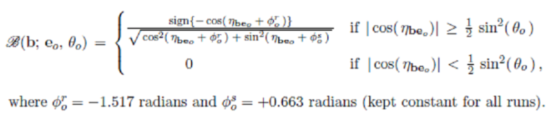
So Mathematica version is not perfect. You are right of course about the prediction of my analytical model. But it would be nice also to get the simulation as perfect as possible. And in that regard I have made a mistake in the prescription I posted above. I forgot the square-root in the denominator. The correct prescription is this:

[FrediFizzx]

HI Joy,

A fix for a better computer simulation would be to not have the zeros go into the A and B outputs then only average over the total number of valid outputs that you do end up with since those zero states don't exist in Nature to begin with. Another slight problem (that you never answered my question on) is that the Sign function outputs zero if the -cos is zero. That should either go to be +1 or -1. But which one? Or doesn't matter? It is easiest to make it go to -1. And of course the program could be setup to do 0.1 degree increments instead of 1 degree increments. A lot of the foregoing is beyond my current capabilities but eventually I could do it with some help.

[Joy Christian]

HI Joy,

A fix for a better computer simulation would be to not have the zeros go into the A and B outputs then only average over the total number of valid outputs that you do end up with since those zero states don't exist in Nature to begin with. Another slight problem (that you never answered my question on) is that the Sign function outputs zero if the -cos is zero. That should either go to be +1 or -1. But which one? Or doesn't matter? It is easiest to make it go to -1. And of course the program could be setup to do 0.1 degree increments instead of 1 degree increments. A lot of the foregoing is beyond my current capabilities but eventually I could do it with some help.

Hi Fred,

Sorry I missed your question earlier. If I understand you correctly, you are asking what happens when the argument of -cos is a multiple of pi/2, in which case -cos(pi/2) = 0, so what value should the sign{-cos(pi/2)} be assigned? Is that what you are asking? If so, then the answer is 0. sign function outputs only two values, +1 or -1, by definition. So sign{-cos(pi/2)} gives 0, not +1 or -1. Have I understood your question correctly?

[FrediFizzx]

But the problem in the computer simulation is that only +/-1 should go to the A and B results. Not zero. So the Sign function as far as the computer simulation goes should not output zero. This is probably not a big problem since you probably don't hit exactly zero very often for -cos(x).

[Joy Christian]

But the problem in the computer simulation is that only +/-1 should go to the A and B results. Not zero. So the Sign function as far as the computer simulation goes should not output zero. This is probably not a big problem since you probably don't hit exactly zero very often for -cos(x).

Yes, that is correct. The probability of hitting zero is negligible, so you have to simply find a way to ignore those cases. Including or excluding them would not make any statistical difference. So, in fact, you can just choose them to be -1, since it seems to be convenient for you to do so.