SciPhysicsForums.com

by **Joy Christian** » Wed Feb 12, 2014 2:37 pm

As some of you may know, I have written up a very simple two-page proof of Einstein's local realism: http://libertesphilosophica.info/blog/w ... 1/EPRB.pdf.

Bell's theorem supposed to have proved that it is impossible to produce the EPR-Bohm correlation purely locally, with or without determinism. But the above model proves otherwise (I thank Michel Fodje and John Reed for producing the cited simulations of the model). Further details of the proof, an extensive discussion on the origins of *ALL* quantum correlations, and the specifics of an experimental test of my hypothesis, can be found on my blog: http://libertesphilosophica.info/blog/.

It is very important to realize that the above simple proof of local realism is the end of the road for Bell's theorem. There is no way out for the supporters of Bell's theorem. Let me explain this for the benefit of those unfamiliar with the subject and those who are declining to see the logical power of elementary mathematics:

Bell's argument is exceedingly simple to understand. He argued that no functions of the form A(a, L) = +1 or -1 and B(b, L) = +1 or -1 can reproduce the EPR-Bohm correlation. Here a and b are local experimental parameters, chosen freely by Alice and Bob, who are space-like separated from each other, and L is a common cause shared by both of them. Thus L is a hidden variable, or initial state, or complete state, that deterministically determines the outcomes A and B of the measurements made by Alice and Bob. It is not difficult to see that the functions A(a, L) = +1 or -1 and B(b, L) = +1 or -1 are manifestly local. A(a, L) does not depend on either b or B, and likewise B(b, L) does not depend on either a or A. Moreover, L can be anything one wants. It can be a single variable, or a set of variables, or even a mixed set of discrete or continuous functions. It simply does not matter what L is, as long as it remains confined to the overlap in the backward light-cones of Alice and Bob (cf. the figure in my two-page proof linked above). So, as you can see, nothing can be more clear and transparent than the locality of the functions A(a, L) and B(b, L).

Now, as I noted, Bell's claim is that no such functions can reproduce the EPR-Bohm correlation predicted by quantum mechanics. More precisely, Bell claimed that the product moment E(a, b) = 1/n Sum_i^n { A(a, L^i) B(b, L^i) } cannot be equal to -cosine(a, b) for any such functions A(a, L) and B(b, L), no matter how large the n is.

But it is not difficult to see from the two-page document linked above that this claim is simply false. You might better appreciate what I am saying if you take a look at this supporting document: http://libertesphilosophica.info/blog/w ... mplete.pdf. But even without the backing of this document it is quite easy to see from my two-page proof that Bell's claim is simply wrong. You may now wonder why, then, is there still so much determined resistance to accept this elementary mathematical demonstration? Well, to understand that you may have to consult some sociologists of science. Or better still, read "The Golem" by Harry Collins and Trevor Pinch.

Joy Christian

by **gill1109** » Wed Feb 12, 2014 9:55 pm

I understand that $a$ , $b$ , $x$ and $e_0$ can be represented by elements of $S^2$ , the set of unit vectors in $R^3$ . The cosine of the angle between directions $x$ and $e_0$ is then equal to the inner-product $x^T e_0$ . I understand that we may assume $\theta_0 \in [0,\pi/2]$ .

It follows that

$\Lambda = S^2 \times \{0\}$

since for any $\theta_0 > 0$ and any $e_0$ , there exists $x$ with $|x^T e_0}| < \frac12 \sin^2(\theta_0)$ . In particular, any $x$ perpendicular to $e_0$ does the job.

by **Joy Christian** » Wed Feb 12, 2014 10:50 pm

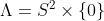
There are infinitely many independent 2-spheres within a 3-sphere. More precisely, there are 1-sphere worth of 2-spheres within a 3-sphere: 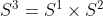$S^3 = S^1 \times S^2$ , at least locally, at each point. The physical 3-space in my model is $S^3$ , not $R^3$ . According to my model $R^3$ are only infinitesimal tangent spaces at each point of $S^3$ .

The constraint $|x^T e_0| \geq \frac{1}{2} \sin^2(\theta_0)$ follows from the triangle inequality for unit quaternions, where $e_0$ is a random vector and $\theta_0$ is an independent random scalar: http://libertesphilosophica.info/blog/w ... mplete.pdf. The correct set $\Lambda$ of the complete states $(e_0, \theta_0)$ is derived, within $S^3$ , in equation (11) of this document.

by **gill1109** » Thu Feb 13, 2014 12:48 am

Ah, the Math of Joy!

I think I begin to get it. In Minkwe's simulation, $e_0$ is chosen at random from the 0-sphere $S^1$ . The tangent space therefore looks at every point like $S^0$ . All points of $S^0$ are represented on Alice's side by $\pm a$ and on Bob's side by $\pm b$ .

That makes a kind of sense. Like poetry.

by **gill1109** » Thu Feb 13, 2014 3:22 am

Now I would like to understand how to "lift" Minkwe's simulation to $S^2$ . After all, we can in principle measure the spin of two particles in any two directions $a, b \in R^3$ .

I fix the length of these vectors (which are only used to define directions) at 1.

So the measurement settings can be taken to be two points $a, b \in S^2$ , represented by unit vectors in $R^3$ . According to "complete.pdf" the state of the pair of particles is described by three points $x, e_0, g_0 \in S^2$ . They have to satisfy certain constraints and anyway, we don't need the complete information of the three points, we just need to know $e_0 \in S^2$ and $\theta_0 = \eta(g_0, x) = g_0 ^\top x$ .

It is unclear to me why we are starting with two completely different unit vectors $e_0, g_0 \in S^2$ , and whether $x \in S^2$ is a fixed property of the state or some kind of dummy variable or local coordinate. But anyway, we proceed: this is the Math of Joy.

The constraints are that $|x^\top e_0| \ge {\scriptstyle\frac 12} \sin^2(\theta_0)$ where on Alice's side, $x = a$ , and on Bob's side, $x = b$ . It's not stated explicitly but I suppose that the idea is that to generate one pair of particles and one pair of measurement outcomes, one does the following:

Alice and Bob choose settings $x = a$ and $x = b$ .

Repeatedly, we pick independently and uniformly, $e_0 \in S^2$ and $\theta_0 \in [0,\pi/2]$ , testing every time the two conditions $|x^\top e_0| \ge {\scriptstyle\frac 12} \sin^2(\theta_0)$ where on Alice's side, $x = a$ , and on Bob's side, $x = b$ . If both conditions are satisfied, we have been successful in having generated one state, and we proceed to deliver the two measurement outcomes $A = - \text{sign} (a^\top e_0)$ and $B = \text{sign} (b^\top e_0)$ .

It is obviously child's play to simulate this model, and anyone with an appetite for trigonometry and calculus can also do the calculations to figure out the joint probability distribution of the two outcomes given the two settings. I shall report on a simulation experiment later. It did not give me the singlet correlations but it did give me a violation of CHSH. I suspect that in order to reproduce the singlet correlations exactly we need to sample $\theta_0$ from a different distribution and/or adapt the rejection/acceptance criteria.

Note for Joy: regarding formula (13), in good mathematical typography the function "sign" should be set in Roman text, not in italic math symbols, c.f. "log", "sin" and so on. Secondly, in view of the definition of the domain $\Lambda$ , the second line of (13) is superfluous and indeed misleading. The outcomes of measurements are +/-1. There never is an outcome "0" because there wouldn't have been a state if the outcome had been 0.

by **Joy Christian** » Thu Feb 13, 2014 4:39 am

gill1109 wrote:...regarding formula (13), in good mathematical typography the function "sign" should be set in Roman text, not in italic math symbols, c.f. "log", "sin" and so on. Secondly, in view of the definition of the domain $\Lambda$ , the second line of (13) is superfluous and indeed misleading. The outcomes of measurements are +/-1. There never is an outcome "0" because there wouldn't have been a state if the outcome had been 0.

Thank you for your suggestion. I have changed the font of "sign" to Roman font. I am, however, keeping the second line of (13) as it is, because it was added after a question raised by Lucien Hardy when he first saw the prescription last year. He asked: What happens when $|x^T e_0| < \frac{1}{2} \sin^2(\theta_0)$ ? Well, nothing happens. There is a more detailed discussion about this ambiguity in notation in this chapter: http://libertesphilosophica.info/blog/w ... hapter.pdf [cf. eqs. (A.9.48) and (A.9.49) on page 254 and eqs. (A.9.53) and (A.9.54) on page 256]. The difference between these two sets of prescriptions is the difference between ontology and computability.

by **gill1109** » Thu Feb 13, 2014 6:05 am

Apologies for posting this in two threads simultaneously:

Here are links to html notebooks of my implementation in R of the the two-dimensional (S^1, subset of R^2) version of Minkwe's implementation of Christian's model

http://rpubs.com/gill1109/13269

and of a new three-dimensional version (S^2, subset of R^3)

http://rpubs.com/gill1109/13270

The other posting is in the thread "Computer Simulation of EPR Scenarios" at

viewtopic.php?f=6&t=11&p=161#p161

by **gill1109** » Thu Feb 13, 2014 6:13 am

Joy Christian wrote:Lucien Hardy ... asked: What happens when $|x^T e_0}| < \frac12 \sin^2(\theta_0)$ ? Well, nothing happens. There is a more detailed discussion about this ambiguity in notation in this chapter: http://libertesphilosophica.info/blog/w ... hapter.pdf [cf. eqs. (A.9.48) and (A.9.49) on page 254 and eqs. (A.9.53) and (A.9.54) on page 256]. The difference between these two sets of prescriptions is the difference between ontology and computability.

My answer would have been: "it doesn't happen".

IMHO, this is not an ambiguity of notation, but an abuse of notation, since you are talking about the value taken by a function when supplied with an argument which is outside of its domain. I would say that strictly speaking the left hand side is "undefined". We cannot say "it equals 0".

Well, there can be good pedagogical reasons to abuse notation... still I would have preferred to see ... = "undefined", not ... = 0.

If we are talking about computability, a decent computer language also allows a variable to take a value outside of its declared range, which then might be denoted by "NA" (not available). In R for instance, "real numbers" can even equal +/- Infinity and Nan ("not a number" - the result of 0/0, for instance), as well as genuine real numbers and as well as being "NA". There are on the other hand only finitely many different real numbers.

All this according to pretty universally agreed IEEE and ACM standards which are implemented in all decent floating point hardware.

by **Joy Christian** » Thu Feb 13, 2014 6:36 am

gill1109 wrote:My answer would have been: "it doesn't happen".

Fine with me. The bottom line is that there exist no states for which $|x^T e_0}| < \frac12 \sin^2(\theta_0)$ for any $x$ , so the question of corresponding outcomes does not arise.

by **gill1109** » Thu Feb 13, 2014 7:42 am

Joy Christian wrote:Fine with me. The bottom line is that there exist no states for which $|x^T e_0}| < \frac12 \sin^2(\theta_0)$ for any $x$ , so the question of corresponding outcomes does not arise.

In Minkwe's simulation, states are created for which $|a^\top e_0}| \ge \frac12 \sin^2(\theta_0)$ and $|b^\top e_0}| \ge \frac12 \sin^2(\theta_0)$ , but for many other values of $x$ , it will be true that $|x^\top e_0}| < \frac12 \sin^2(\theta_0)$ . In fact, if $\theta_0 > 0$ , there are no $e_0\in S^2$ at all for which $|x^\top e_0}| \ge \frac12 \sin^2(\theta_0)$ for all $x\in S^2$ .

by **Joy Christian** » Thu Feb 13, 2014 8:30 am

There are infinitely many $S^2$ within $S^3$ , not just one fixed $S^2$ within one fixed $R^3$ . As far as I can see Michel has implemented this state of affairs correctly.

by **gill1109** » Thu Feb 13, 2014 1:04 pm

I know. I already commented on this a while ago.

Perhaps then you can comment on the two simulations I have just posted: one is a "copy" of Michel's (hopefully a "true" copy), the other "converts" Michel's scheme from $S^1$ to $S^2$ . Both exhibit strong violations of CHSH but in fact the sample sizes in my simulation are large enough that we can be certain that neither model reproduces the singlet correlation (cosine difference of angles ...). They are both systematically off target, the "full" simulation $S^2$ is further off than the restricted one, Michel's original, $S^1$ .

My provisional conclusion: either your analytical model calculations are "wrong", or Michel's code does not simulate your model but simulates something else instead.

This is why I asked many times for you to provide us with a short set of unambiguous "programmer's instructions", just as Michel himself gave us not only computer code but also a succinct description of the algorithm he has implemented. I am still waiting. You keep saying that you can't program so you can't check Michel's code, yet you seem to know it is correct. Yet it is perfectly clear that it does not match your model predictions. So are you going to blame Michel for that but give no guidance how he should fix his *algorithm*? You don't have to explain to him how to fix his *code*.

Similarly my two simulations: are you going to tell me what is wrong in the algorithm I am using?

The advantage of R over Python is that the number of lines of code is about the same as the number of lines of a concise but complete description of the algorithm. If you need help "decoding" R language I would be happy to add a line by line explanation of what is going on.

For instance:

rnorm(3) means a vector of length 3 of standard normal variates.
runif(N, 0, pi/2) means a vector of length N of uniform random numbers between 0 and pi/2
If x is a vector then x * x means the vector of squares of elements of x; sin(x) means the vector of sines of elements of x, and so on.
That's about all you need to know.

by **gill1109** » Thu Feb 13, 2014 1:26 pm

PS We see that Christian's "simple two-page proof" does strongly depend on "the Math of Joy": when he writes $\forall x$ he doesn't mean "for all (every) x" at all; he means for any one particular x which suits him at any particular moment. This kind of creative mathematics also permeated "Christian 1.0", the earlier version of Joy's model, as exemplified in the famous "one page paper" of some years back. This is why computer verification of Christian's claims is such a powerful tool: ambiguity is no longer tolerated.

by **Joy Christian** » Thu Feb 13, 2014 1:58 pm

gill1109 wrote:Perhaps you can comment then on the two simulations I have just posted: one is a copy of Michel's, the other "converts" Michel's scheme from $S^1$ to $S^2$ . Both exhibit strong violations of CHSH but in fact the sample sizes in my simulation are large enough that we can be certain that neither model reproduces the singlet correlation (cosine difference of angles). They are both systematically off target, the "full" simulation $S^2$ is further off than the restricted one $S^1$ .

Conclusion: either your model is "wrong", or Michel's code does not simulate your model, but something else instead.

That is your conclusion, based on your simulation. I do not trust your simulation. I trust Michel's simulation, and its translation by John Reed. All Michel has done differently from me in his simulation is that he has used a streamlined notation. He has not changed anything in my model. He is still working in full $S^2 \in S^3$ .
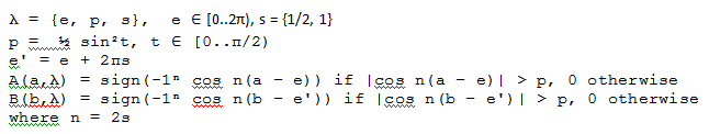
He has not shifted to $S^1$ or anything else. It is clear that I will have to take baby steps with you to make you see this. So let us have a look at Michel's notation:

Now, note that his prescription is in fact slightly more general than mine. His prescription reduces to mine for s = 1/2, n = 1. This much should be easy for you to understand. Next, let us look at his notation in the function $|\cos(a - e)|$ , where $a$ and $e$ are scalars. But does this make his scheme reduce to $S^1$ as you claim? Absolutely not. His number $\cos(a - e)$ is exactly the same as my number $\cos(\eta_{{\bf a}{\bf e}_o})$ . The difference is only in notation, not in the scheme. It shouldn't make any difference whether one uses Michel's notation or mine. And yet you claim a difference. That proves to me that you have done something wrong. You have not been able to reproduce the simulations of Michel Fodje and John Reed cited in this document.

I will not be bothered to comment on your continued propaganda about your inability to understand the mathematics in my one-page paper or two-page document.

by **gill1109** » Thu Feb 13, 2014 2:29 pm

Joy, my R code is a precise implementation of Michel's algorithm: his description of what his code does. And as far as I can see his description is correct - his code does do that. My code does the same.

Yes I know that his code actually generalizes your model in several ways.

Why do I say that his code is a version of your model based on $S^1$ instead of $S^2$ ? You have put your finger on the key point: $|\cos(a-e)|$ . In his code, a and e are angles between 0 and 2 pi. Yes, the absolute value of the cosine of the difference can also be considered to be the same as $\cos(\eta_{a e_0})$ in your writing. However, his a and e_0 are not unit vectors in $R^3$ but unit vectors in $R^2$ . In particular the part coming from the state: he selects e_0 according to a uniform probability distribution over $S^1$ while your text implies a uniform probability distribution over $S^2$ .

My R code is very simple to read. I hope that others (in particular, "minkwe") will take a look, and test it. I have been able to reproduce exactly the simulations of Michel. They do give results systematically slightly different from the singlet correlation, provided one implements his algorithm with higher numerical precision and with larger sample sizes. Note for instance that he simulated e_0 by sampling from a discrete uniform distribution, not from a continuous uniform distribution.

Indeed I do not understand your mathematics as mathematics. I am beginning to understand it as poetry. This could be "my fault" - it is not necessarily a criticism of your writing. I just like to share my experiences with others, to find out if others have the same difficulties as I do. After all, the title of this thread, started by you, is "a simple two-page proof of local realism". I suppose you are inviting discussion of the proof by others. Is it really so simple?

by **Joy Christian** » Thu Feb 13, 2014 4:08 pm

gill1109 wrote:They do give results systematically slightly different from the singlet correlation, provided one implements his algorithm with higher numerical precision and with larger sample sizes.

OK, I know what the problem is. In Michel's simulation, in order to prevent Alice and Bob both ending up detecting the same particle, he has introduced a phase-shift of $\pi$ between the functions A(a; e, t) and B(b; e, t). If you now want to randomly choose all three vectors, a, b, and e, on $S^2$ instead of $S^1$ , then you would have to introduce a nontrivial phase-shift instead of just $\pi$ . This should remain constant throughout the experiment. It would be what Bell used to call a non-hidden variable.

by **gill1109** » Thu Feb 13, 2014 9:52 pm

Here is the core piece of code from http://rpubs.com/gill1109/13269 and http://rpubs.com/gill1109/13270
Please explain what phase needs to be introduced to lift from S1 to S2. Actually: the S2 version seems spot-on, the S1 version is slightly off!

Code: Select all: alpha <- 0 *2* pi / 360 ## CHSH: try 0 and 90 degrees beta <- 45 *2* pi / 360 ## CHSH: try 45 and 135 degrees a <- c(cos(alpha), sin(alpha)) ## S2 version: c(cos(alpha), sin(alpha), 0) b <- c(cos(beta), sin(beta)) ## S2 version: c(cos(beta), sin(beta), 0) sumprod <- 0 N <- 0 for (i in 1:10^6) { e0 <- rnorm(2) ## S2 version: rnorm(3) e0 <- e0/sqrt(sum(e0^2)) theta0 <- runif(1, 0, pi/2) ca <- sum(e0*a) cb <- sum(e0*b) s <- (sin(theta0)^2)/2 if (abs(ca) > s & abs(cb) > s ) { sumprod <- sumprod + sign(ca)*sign(cb) N <- N+1 } } sum(a*b) ## Theoretical correlation N ## Number pairs of particles sumprod/N ## Observed correlation

Here is a typical output

Code: Select all: > sum(a*b) ## Theoretical correlation [1] 0.7071068 > N ## Number pairs of particles [1] 690569 > sumprod/N ## Observed correlation [1] 0.700198

The difference (0.700 instead of 0.707) is significant and systematic.

However in S2 we get, typically:

Code: Select all: > sum(a*b) ## Theoretical correlation [1] 0.7071068 > N ## Number pairs of particles [1] 601609 > sumprod/N ## Observed correlation [1] 0.7071985

by **gill1109** » Fri Feb 14, 2014 2:41 am

Faster, bigger, better... here are two simulations, one for the S^1 model, one for the S^2 model. The S^2 model comes much closer to the singlet correlations than the S^1 model but definitely does not reproduce them exactly. No need to do the trigonometry to *prove* they are different ...

First the S^1 model, i.e., Minkwe algorithm, which we could also call Caroline Thompson's chaotic disk with Joy Christian's choice of probability distribution of "theta_0"

Code: Select all: alpha <- 0 * 2* pi / 360 beta <- 45 * 2 * pi / 360 a <- c(cos(alpha), sin(alpha)) b <- c(cos(beta), sin(beta)) M <- 10^8 t <- runif(M, 0, 2*pi) x <- cos(t) y <- sin(t) e <- rbind(x,y) ca <- colSums(e*a) cb <- colSums(e*b) theta <- runif(M, 0, pi/2) s <- (sin(theta)^2) / 2 good <- abs(ca) > s & abs(cb) > s N <- sum(good) corr <- sum(sign(ca[good])*sign(cb[good]))/N

Result:

Code: Select all: > corr [1] 0.6995283 > sqrt(1/N) [1] 0.0001203852 > sum(a*b) [1] 0.7071068

The simulated correlation is 0.6995 +/- 0.0001 while the theoretical correlation is 0.7071.

Now the S^2 version, i.e., Caroline Thompson's chaotic ball with Joy Christian's choice of probability distribution of "theta_0":

Code: Select all: alpha <- 0 * 2 * pi / 360 beta <- 45 * 2 * pi / 360 a <- c(cos(alpha), sin(alpha), 0) b <- c(cos(beta), sin(beta), 0) M <- 10^8 z <- runif(M, -1, 1) t <- runif(M, 0, 2*pi) r <- sqrt(1 - z^2) x <- r * cos(t) y <- r * sin(t) e <- rbind(x,y,z) ca <- colSums(e*a) cb <- colSums(e*b) theta <- runif(M, 0, pi/2) s <- (sin(theta)^2) / 2 good <- abs(ca) > s & abs(cb) > s N <- sum(good) corr <- sum(sign(ca[good])*sign(cb[good]))/N

Result:

Code: Select all: > corr [1] 0.7052408 > sum(a*b) [1] 0.7071068 > sqrt(1/N) [1] 0.0001289189

The simulated correlation is 0.7052 +/- 0.0001 while the theoretical correlation is 0.7071.

by **gill1109** » Fri Feb 14, 2014 9:44 am

OK, so it is now established that Michel Fodje (minkwe)'s simulation based on picking e_0 from S^1 does not exactly reproduce the cosine correlation we are after. Neither does an S^2 simulation, though it comes a little bit closer. The S^2 simulation is a special case of Caroline Thompson's chaotic/rotating ball model with circular caps of varying diameter:

Now the strange thing is, how did Christian arrive at the particular choice f(theta_0) = 1/2 sin^2(theta_0) together with theta_0 uniformly distributed over [0, pi/2]. These two ingredients determine the probability distribution of the circular caps in the rotating ball model. According to his documents EPRB.pdf and complete.pdf, the choice for the function f(.) is essentially arbitrary, it just has to be chosen to satisfy certain bounds coming from the triangle inequality for quaternions. theta_0 is supposed to represent the angle between x and g_0 where neither x nor g_0 are further specified in those documents, so why theta_0 should be taken uniform on [0, pi/2] is another mystery. If x and/or theta_0 are picked uniformly at random in S^2, the angle between the two does *not* have the uniform distribution. (At a uniform random point of the sphere, longitude is uniformly distributed, but latitude isn't).

However the simulations show that these "arbitrary" choices are extraordinarily well made, though not well enough to give us the cosine correlations, exactly. So how does he do it? Someone who has studied, and tried to refine, Caroline Thompson's model might come across these two choices, by a process of trial and error. There is no way they can be "derived" by some exact principles, since they only deliver an approximation to what we are after.

by **Joy Christian** » Fri Feb 14, 2014 2:40 pm

gill1109 wrote:OK, so it is now established that Michel Fodje (minkwe)'s simulation based on picking e_0 from S^1 does not exactly reproduce the cosine correlation we are after. Neither does an S^2 simulation....

It should be noted that all Gill has managed to establish is that he has not been able to reproduce Michel's simulation either as competently or as correctly as both Michel and John Reed have been able to.

Those who are familiar with his past failures would also recognize that he has a tendency to get carried away with his own misconceptions rather than recognizing that he has actually failed to understand what he is analyzing. More to the point, anyone who has actually bothered to study my longer paper linked above would have noticed that the simulations by Chantal Roth and Michel Fodje in fact complement each other rather nicely. Each simulation exhibits a different representation of one and the same geometrical and topological structure of the 3-sphere. There is no mystery to why both simulations exactly reproduce the singlet correlation, albeit appearing at first sight to be quite different. As I have stressed many times before, EPR-Bohm correlations are correlations among the points of a parallelized 3-sphere. Of course if the flatlanders would rather continue to view these correlations in a primitive way from their perspective of $R^3$ instead of $S^3$ , then I cannot help them. But any one who has actually bothered to read and understand my paper (which discusses both simulations extensively) would not fall for the grotesque straw-man Gill is trying to conjure up.

PS: Here is the longer paper I referred to: http://libertesphilosophica.info/blog/w ... hapter.pdf

SciPhysicsForums.com

A simple two-page proof of local realism

A simple two-page proof of local realism

Re: A simple two-page proof of local realism

Re: A simple two-page proof of local realism

Re: A simple two-page proof of local realism

Re: A simple two-page proof of local realism

Re: A simple two-page proof of local realism

Re: A simple two-page proof of local realism

Re: A simple two-page proof of local realism

Re: A simple two-page proof of local realism

Re: A simple two-page proof of local realism

Re: A simple two-page proof of local realism

Re: A simple two-page proof of local realism

Re: A simple two-page proof of local realism

Re: A simple two-page proof of local realism

Re: A simple two-page proof of local realism

Re: A simple two-page proof of local realism

Re: A simple two-page proof of local realism

Re: A simple two-page proof of local realism

Re: A simple two-page proof of local realism

Re: A simple two-page proof of local realism

Who is online