Metric Topology and the Origins of Quantum Correlations

[Joy Christian]

Since 2007 I have argued that the strong (or "quantum") correlations we observe in Nature are entirely topological effects, originating from the very topology of the physical space we live in [ cf. discussions in my book ; see also "Topology", by James R. Munkres (2000) ]. In other words, the so-called "quantum" correlations have nothing to do with the bizarre notions like "quantum entanglement", or "non-locality", or "non-reality", or "irreducible randomness", as some would have us believe.

Now one of the most important ways of imposing topology on a set -- such as a set of events taking place in a physical space -- is to define the topology in terms of a metric on the set. Such a topology on the set is then called metric topology. Thus we can discuss the origins of quantum correlations in terms of a metric topology.

It turns out that ALL quantum correlations, no matter how complicated, can be understood local-realistically in terms of a metric topology, as correlations among the points of a parallelized (or octonionic) 7-sphere [ cf. the theorem on page 13 of my book linked above ]. For simplicity and definiteness, however, let us concentrate on the simplest quantum correlation, namely the EPR-Bohm or singlet correlation --- i.e., let us try to understand this emblematic correlation locally, in terms of the metric topology of the three-dimensional physical space, without worrying about the higher-dimensional space needed to represent the octonions correctly. But even for this 3D case ( involving the simple rotationally invariant singlet state ) we cannot escape the fact that rotational and spinorial properties of the physical space can be modelled correctly only by using quaternionic numbers. As Grassmann, Hamilton, and Clifford discovered long time ago, ordinary tensors are simply not capable of performing this feat correctly. What is required to model the physical space correctly is a certain combination of scalars and bivectors in the form of unit quaternions. More precisely, we must model the physical space as a set of unit quaternions, which is just a parallelized 3-sphere, or S^3, as described, for example, in this paper.

Now a quaternionic S^3, which is locally (or tangentially) identical to R^3, happens to be "flat" as far as its Riemann curvature is concerned. It is thus quantifiable by the familiar Euclidean metric tensor, . Its geometrical and topological properties are entirely describable by intrinsic torsion, which is a tensor "attached" to every point of S^3. In other words, in the quaternionic guise the metric topology of S^3 is rather trivial. But of course its intrinsic torsion, although constant at every point, is highly non-trivial, and gives rise to the quantum (or EPR-B) correlation. I have described how this comes about far too many times in many papers to repeat the derivation here once again, but the details can be found in Eqs. (18) to (26) of this paper. The quantum correlations are then derived explicitly in the Eq. (B10).

It is very important to recognize here that what Eq. (B10) proves is simply , where and

This result follows simply and elegantly because we have correctly used the Clifford-algebraic or quaternionic representation of the 3-sphere to model rotations. But suppose we now insist on using ordinary vectors and the corresponding non-Clifford-algebraic representation of S^3 to model rotations. Can we still derive the strong correlation ? It may seem that the answer would have to be no, because, as noted, ordinary tensors like vectors are not capable of modelling rotations in the physical space correctly ( let alone modelling spinors in a singularity-free manner ). Recall, however, that within the present context of Bell's theorem we are not interested in modelling all possible rotations and their all possible compositions in the physical space. We are only interested in establishing the correct correlation between some very special limiting points of the 3-sphere, namely between its scalar points, such as and .

It turns out that in that case we can indeed model rotations (or more precisely, their spin values) by means of ordinary vectors and their inner products. The resulting space however has a metric-like structure that is no longer Euclidean -- i.e., it is no longer "flat" in the usual sense, and the role played by torsion within S^3 becomes obscure. In fact, a single Riemannian metric is not capable of modelling this space. An entire spectrum of effective metrics are required to model the rotation or spin values correctly, as originally discovered by Michel Fodje ( although his approach was phenomenological rather than geometrical or topological ). Given two vectors and , their inner product is defined by the constraint , with the two extreme cases, namely and quantifying the weakest and the strongest topologies, respectively. Here the weakest topology dictated by the constraint is the familiar topology of R^3, where relatively few vectors and are orthogonal to each other. The strongest topology dictated by , on the other hand, is more interesting, since in that case nearly all vectors and are orthogonal to each other. All intermediate topologies are dictated by the effective metric





Here the generalized orthogonality of the vectors and is defined, evidently, by the condition , and it depends on the parameter .

I have explained the detailed relationship between the Clifford-algebraic representation of the 3-sphere and the above effective representation in terms of ordinary vectors in this paper. A further, more direct relationship between the two representations is derived in Eq. (B10) of this paper. It can also be seen explicitly in one of the three different ways the EPR-B correlation has been calculated in this simulation. Let me reproduce here the essential part of the code in the simulation to show the simplicity of the effective representation described above. The measurement functions of Alice and of Bob generated in the simulation are exactly the local functions demanded by Bell in his 1964 paper, and the correlations are then calculated using the coincidence counts in exactly the same manner as in the actual experiments. The displayed graphs put to rest any lingering doubt that there might be somehow some uncounted "0 outcomes" in the simulation. But in the 3-sphere there are no "0 outcomes", as is evident from Eq. (B10) of this paper consolidating the analytical model:

Code: Select all

A = +sign(g(a,e,s))  # Alice's measurement results A(a, e, s) = +/-1  # Here g(u,v,s) is a metric on S^3, reducing to the usual g on R^3
B = -sign(g(b,e,s))  # Bob's measurement results B(b, e, s) = -/+1    # A(a, L) = +/-1 and B(b, L) = +/-1 are exactly as defined by Bell
     
Cuu = length((A*B)[A > 0 & B > 0])   # Coincidence count of (+,+) events
Cdd = length((A*B)[A < 0 & B < 0])   # Coincidence count of (-,-) events
Cud = length((A*B)[A > 0 & B < 0])   # Coincidence count of (+,-) events
Cdu = length((A*B)[A < 0 & B > 0])   # Coincidence count of (-,+) events
       
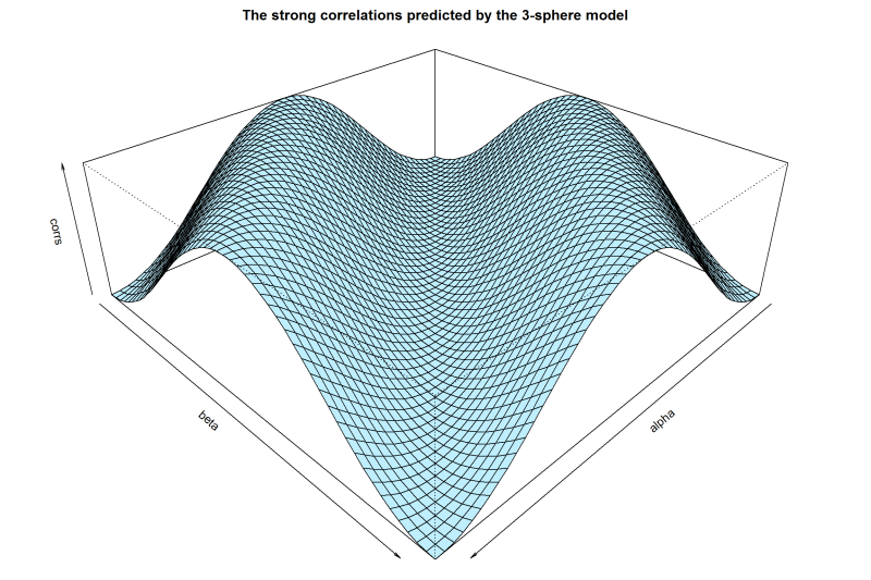
corrs[i,j] = (Cuu + Cdd - Cud - Cdu) / (Cuu + Cdd + Cud + Cdu) # = -a.b

# There are no "0 outcomes" within S^3: Cou = Cod = Cuo = Cdo = Coo = 0
CoB = length(A[g(a,e,s) & A == 0])   # Number of A = 0 events within S^3 (regardless of B events) = 0
CAo = length(B[g(b,e,s) & B == 0])   # Number of B = 0 events within S^3 (regardless of A events) = 0


Finally, I have built this simplified version of the simulation which can be useful for testing the spectacular effects of topology changes when the stochastic parameter is changed in succession. Leaving everything else unchanged in the code, simply set , , , and , successively, to see how the correlations change from linear correlation to box correlation. The quantum correlations are then exactly reproduced for a uniform distribution of topologies!

Joy Christian

[Brad]

Hi Joy, doesn't this theory imply that a particle may change some aspect of itself dependent on the nature of the spacetime it finds itself in. That is, within a void (where expansion occurs) some quantum aspect of a particle would be different than that same aspect would appear to us within the static spacetime of our gravitational fields. How would Einstein compare this to Weyls' Gauge theory that he rejected because a particles nature would be dependent on its history?
Thanks, Brad.

[Joy Christian]

Hi Joy, doesn't this theory imply that a particle may change some aspect of itself dependent on the nature of the spacetime it finds itself in. That is, within a void (where expansion occurs) some quantum aspect of a particle would be different than that same aspect would appear to us within the static spacetime of our gravitational fields. How would Einstein compare this to Weyls' Gauge theory that he rejected because a particles nature would be dependent on its history?
Thanks, Brad.

Hi Brad,

Thanks for your question. It is a very good question.

If the nature of a particle is dependent on its history then that would indeed be a worry, and I would reject the model just as Einstein rightly rejected Weyl's theory.

We have to unpack the model to see what is going on. In the effective description the metric g(a; e, s) does depend on the initial state (e, s) of the particle. For different initial states (e, s) the effective metric g(a; e, s) is different. But this is an artefact of the effective description. In the original Clifford-algebraic model there is no such dependence. There the metric of the space is independent of the initial state, , of the particle. Thus, just as non-locality is an illusion stemming from an incorrect (or non-Clifford-algebraic) modelling of the physical space, the apparent dependence of the nature of the particle on its history is also an illusion.

I hope this answers your question. If it does not, then please feel free to press me on this again, because this is something that needs to be unpacked more clearly.

[FrediFizzx]

If the nature of a particle is dependent on its history then that would indeed be a worry, and I would reject the model just as Einstein rightly rejected Weyl's theory.

Why is that a worry? Perhaps a more specific example would be good here if someone can offer one up?

[Ben6993]

FrediFizzx on Thu Aug 13, 2015 8:08 am wrote

Joy Christian wrote:
If the nature of a particle is dependent on its history then that would indeed be a worry, and I would reject the model just as Einstein rightly rejected Weyl's theory.

Why is that a worry? Perhaps a more specific example would be good here if someone can offer one up?

In my preon model, an electron is created, at say a particle pair creation, and then has constant structure/contents until it is destroyed or reformed at a measurement/interaction.
So within that lifespan of an electron, between interactions, its contents are independent of anything else.
However, the distribution of the contents of an electron may vary, for example the weak isospin contents of an electron may be distributed in space as a field and that field will interact with the weak isospin field of a higgs and cause the electron to have mass. But that would not affect the contents of an electron, merely the distribution and dynamics of the contents.

[FrediFizzx]

In my preon model, an electron is created, at say a particle pair creation, and then has constant structure/contents until it is destroyed or reformed at a measurement/interaction.
So within that lifespan of an electron, between interactions, its contents are independent of anything else.
However, the distribution of the contents of an electron may vary, for example the weak isospin contents of an electron may be distributed in space as a field and that field will interact with the weak isospin field of a higgs and cause the electron to have mass. But that would not affect the contents of an electron, merely the distribution and dynamics of the contents.

What exactly is meant by "contents" and "nature"? Those kind of descriptions seem a little vague to me.

[Ben6993]

FrediFizzx on Thu Aug 13, 2015 6:05 pm wrote

Ben6993 wrote:
In my preon model, an electron is created, at say a particle pair creation, and then has constant structure/contents until it is destroyed or reformed at a measurement/interaction.
So within that lifespan of an electron, between interactions, its contents are independent of anything else.
However, the distribution of the contents of an electron may vary, for example the weak isospin contents of an electron may be distributed in space as a field and that field will interact with the weak isospin field of a higgs and cause the electron to have mass. But that would not affect the contents of an electron, merely the distribution and dynamics of the contents.

What exactly is meant by "contents" and "nature"? Those kind of descriptions seem a little vague to me.

The contents of a left-handed electron. in my preon and hexark model. are A C X1 where A and C are preons. X1 is any neutral pair of preon and anti-preon. So for example A C B B' is a left-handed electron. (See Table 7 on page 6 of http://vixra.org/abs/1505.0076 for the preon content of electrons; Table 2 on page 3 for what preons are; and the Appendix plus pages 1 and 2 for how each preon is constructed out of hexarks.)
A C B B' is a fixed set of entities and will stay unchanged between interactions. At interactions, the preons may swap about [as in chemical formulae eg NaOH + HCl -> NaCl + H2O] so an interaction means the end of one form and the beginning of a new form. A preon never changes its content and neither does a hexark.

I can't find where I have used the word "nature"?

[Ben6993]

Ah, found it. Joy used the word "nature", not me.

Joy Christian wrote on Thu Aug 13, 2015 7:20 am:
If the nature of a particle is dependent on its history then that would indeed be a worry, and I would reject the model just as Einstein rightly rejected Weyl's theory.

(So was that a straw man criticism, Fred??? )

[Mikko]

If the nature of a particle is dependent on its history then that would indeed be a worry, and I would reject the model just as Einstein rightly rejected Weyl's theory.

Why is that a worry? Perhaps a more specific example would be good here if someone can offer one up?

Mainly because nature and intrinsic properties of a particle are observed to be independent of its history. This is best observed of electron. If one electron were any different from the other electrons, an atom containing it would be different from any known atom, which could be observed in its spcectrum and chemical behaviour. For example, sodium with one such electron would be a noble gas. Similar effects are observed about atoms where a muon replaces one of the elctrons (although the shor life-time of muons restricts observation of such atoms).

[FrediFizzx]

Ah, found it. Joy used the word "nature", not me.

Joy Christian wrote on Thu Aug 13, 2015 7:20 am:
If the nature of a particle is dependent on its history then that would indeed be a worry, and I would reject the model just as Einstein rightly rejected Weyl's theory.

(So was that a straw man criticism, Fred??? )

Brad used "nature" also. It wasn't a strawman nor was it any kind of criticism. It was a question. Basically I was thinking of "spin" as far as "nature" or possibly "content" goes.

[Joy Christian]

***
I had a very constructive meeting yesterday with Dr Lucien Hardy of Perimeter Institute who is currently visiting Oxford University. We had a long discussion about a number of problems in foundations of physics, in addition to discussing my latest simulation linked above. He raised a number of concerns about the simulation with penetrating insight. For those who don't know him: He is one of the leading and prominent experts in foundations of quantum mechanics. In the light of his concerns I have revised the latest version of the simulation and cleaned it up substantially. I think this version now addresses most of his concerns: http://rpubs.com/jjc/99993.
***

[Joy Christian]

If the nature of a particle is dependent on its history then that would indeed be a worry, and I would reject the model just as Einstein rightly rejected Weyl's theory.

Why is that a worry? Perhaps a more specific example would be good here if someone can offer one up?

Einstein recommended Weyl's paper for publication, but added a postscript to it in which he points out that in Weyl's theory the frequency of the spectral lines of the atomic clocks would depend on the past and present locations of the atom, contradicting the observed fact that it remains independent of the locations of the atom.

[Joy Christian]

****
Following is the key part in the new version of the simulation: http://rpubs.com/jjc/99993

Code: Select all

A = +sign(g(a,e,s))  # Alice's measurement results A(a, e, s) = +/-1
         
B = -sign(g(b,e,s))  # Bob's measurement results B(b, e, s) = -/+1
       
N = length((A*B)[A & B]) # Number of all possible events observed in S^3
       
corrs[i,j] = sum(A*B)/N  # Product moment correlation coefficient E(a, b)


[Ben6993]

Brad wrote:
Hi Joy, doesn't this theory imply that a particle may change some aspect of itself dependent on the nature of the spacetime it finds itself in. ....

Take a singlet state electron. Joy's model has it inhabiting either a physical space which has trivector -I or a physical space which has +I. If a body has twist + in +I trivector space as viewed by a person in that same space it has twist - in -I trivector space. (And joy's model is supposed to work for macro bodies so we can put a tied observer in a box along with the electron, moving with the electron.) This physical aspect is quite separate from the use of either trivector space as a coordinate system where the physics within a space is independent of the coordinates used. So an electron without inherent chirality could be viewed by its tied observer as having a + or - twist depending on the trivector inhabited by the electron and tied observer. That presumes that light waves do not twist along with the trivectors' twists else the electron would have no chirality in either trivector space?

It seems that there are three aspects now. Inherent chirality (as defined by the toolmaker, see below), twist (from Joy's torsion description) and helicity (as normally defined). Say I make in my flatland workshop a left hand screw and label it L. And I make a right hand screw and label it R. The two screws have inherent chirality L and R. In flatland, I can despatch the two screws around the world and when they are returned to me the L screw will still appear to me to be a left hand screw.

But in 3sphereworld, I can make the L and R screws, though if I and the L screw are in -I space how can I be sure that I am making a genuine L screw or one that only looks like an L because of the -I space we inhabit? Would a nail in flatland look like a screw in -I space? Also, it may be impossible to make an R screw in -I space due to quantum restricions. If I make an R in -I it may look like a 2R when viewed within +I space? It seems that the first definition is irrelevant to Joy's model. That is, the inherent chirality of the electron will be zero. But this will look like a - twist to its tied observer in -I but would look like a + twist to a tied observer in +I (say the two observers are -obs and +obs, respectively).

Say -obs makes an LH screw in -I trivector space in a 3sphereworld workshop, and puts an L label on it. And he also writes L on his left hand. Now move the same observer and screw into a +I space. What will the (now) +obs find? His hand labelled L will still match the chirality of the L screw. But he will presumably realise that Left ain't what t used to be? It looks more like what R used to be?

So to go back to Brad's question, an electron is the same [and seems to me to have inherent chirality zero] when in -I or +I in Joy's model. The LH or RH chiral handedness of an electron, for Joy, is not part of the electron's content but is given by the trivector torsion and is a property of the interaction of the electron with its trivector space. So, just as helicity is not an inherent property of an electron, neither is chirality in Joy's model?

[FrediFizzx]

Brad wrote:
Hi Joy, doesn't this theory imply that a particle may change some aspect of itself dependent on the nature of the spacetime it finds itself in. ....

Take a singlet state electron. Joy's model has it inhabiting either a physical space which has trivector -I or a physical space which has +I. If a body has twist + in +I trivector space as viewed by a person in that same space it has twist - in -I trivector space. (And joy's model is supposed to work for macro bodies so we can put a tied observer in a box along with the electron, moving with the electron.) This physical aspect is quite separate from the use of either trivector space as a coordinate system where the physics within a space is independent of the coordinates used. So an electron without inherent chirality could be viewed by its tied observer as having a + or - twist depending on the trivector inhabited by the electron and tied observer. That presumes that light waves do not twist along with the trivectors' twists else the electron would have no chirality in either trivector space?

It seems that there are three aspects now. Inherent chirality (as defined by the toolmaker, see below), twist (from Joy's torsion description) and helicity (as normally defined). Say I make in my flatland workshop a left hand screw and label it L. And I make a right hand screw and label it R. The two screws have inherent chirality L and R. In flatland, I can despatch the two screws around the world and when they are returned to me the L screw will still appear to me to be a left hand screw.

But in 3sphereworld, I can make the L and R screws, though if I and the L screw are in -I space how can I be sure that I am making a genuine L screw or one that only looks like an L because of the -I space we inhabit? Would a nail in flatland look like a screw in -I space? Also, it may be impossible to make an R screw in -I space due to quantum restricions. If I make an R in -I it may look like a 2R when viewed within +I space? It seems that the first definition is irrelevant to Joy's model. That is, the inherent chirality of the electron will be zero. But this will look like a - twist to its tied observer in -I but would look like a + twist to a tied observer in +I (say the two observers are -obs and +obs, respectively).

Say -obs makes an LH screw in -I trivector space in a 3sphereworld workshop, and puts an L label on it. And he also writes L on his left hand. Now move the same observer and screw into a +I space. What will the (now) +obs find? His hand labelled L will still match the chirality of the L screw. But he will presumably realise that Left ain't what t used to be? It looks more like what R used to be?

So to go back to Brad's question, an electron is the same [and seems to me to have inherent chirality zero] when in -I or +I in Joy's model. The LH or RH chiral handedness of an electron, for Joy, is not part of the electron's content but is given by the trivector torsion and is a property of the interaction of the electron with its trivector space. So, just as helicity is not an inherent property of an electron, neither is chirality in Joy's model?

You are taking Joy's model further than it is meant to be valid. I believe it only works with singlet states. IOW, it is about a system of pairs of particles that had a common creation.

[Ben6993]

Fred wrote:
You are taking Joy's model further than it is meant to be valid. I believe it only works with singlet states. IOW, it is about a system of pairs of particles that had a common creation.

So non-singlet state electrons could live in flatland? And not in S^3?

[Joy Christian]

Fred wrote:
You are taking Joy's model further than it is meant to be valid. I believe it only works with singlet states. IOW, it is about a system of pairs of particles that had a common creation.

So non-singlet state electrons could live in flatland? And not in S^3?

No. For states more general than the singlet state we have to go to S^7, which is a much richer space than S^3 (cf. this paper: http://arxiv.org/abs/1101.1958).

[FrediFizzx]

Fred wrote:
You are taking Joy's model further than it is meant to be valid. I believe it only works with singlet states. IOW, it is about a system of pairs of particles that had a common creation.

So non-singlet state electrons could live in flatland? And not in S^3?

No. For states more general than the singlet state we have to go to S^7, which is a much richer space than S^3 (cf. this paper: http://arxiv.org/abs/1101.1958).

Yeah, that is better. "Valid" was not the correct term to use.

[Ben6993]

Won't the torsion effects be even more exotic in S^7 than in S^3, even for non-singlet electrons?
In my scenario, the "-obs" observer who has written L on his left hand might need to also write TOP on his forehead. When the observer changes to a different torsional space in S^7 he may notice that L ain't what it used to be (it now seems to be R) and TOP ain't what it used to be, too? Which would explain his new headache.

[Joy Christian]

Won't the torsion effects be even more exotic in S^7 than in S^3, even for non-singlet electrons?
In my scenario, the "-obs" observer who has written L on his left hand might need to also write TOP on his forehead. When the observer changes to a different torsional space in S^7 he may notice that L ain't what it used to be (it now seems to be R) and TOP ain't what it used to be, too? Which would explain his new headache.

The intrinsic torsion within S^7 is indeed "more exotic" in S^7 than it is in S^3. Torsion is constant throughout S^3, whereas it varies from point to point within S^7, at least in the manner I have set things up. The non-associativity of octonions is replaced with variable torsion in my set up. But I think Fred's point is that we should not rely too much on intuitive arguments. While the general point you are making is valid, the details of your intuition may not be supported by the mathematics of S^7.