New EPRB simulation using GAViewer
I think Albert Jan Wonnink's new simulation using GAViewer deserves a topic of its own. I have expanded it to the full 360 degrees plus increased the resolution of the output. Here is the code for that.
And the typical results are,
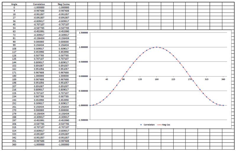
And here is a Excel chart with the data and I added a column for the negative cosine values.
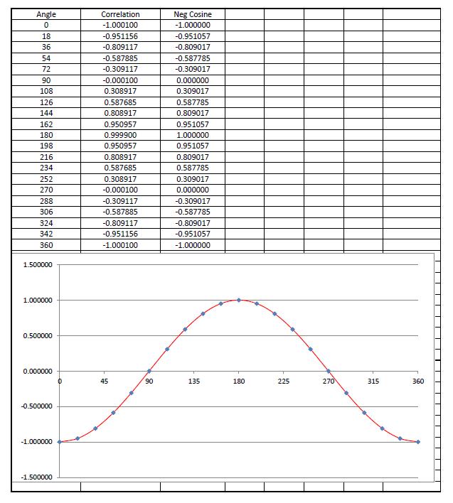
Negative cosine curve is in red and the simulation data points blue. This simulation can be easily expanded to greater resolution.
This definitively proves that Joy's local realistic model is a counter example to Bell's theory.
Is everyone ready for a revolution in physics? !!!
- Code: Select all
function getRandomLambda()
{
     if( rand()>0.5)
{
     return 1;
}
     else
{
     return -1;
}
}

function getVector(idx)
{
     step=0.05*2*pi; //step size is taken 1/10 of pi
     angle=idx*step;
     v=sin(angle)*e1+cos(angle)*e2+0.01*e3;
     return v;
}
     batch test()
{
     set_window_title("Test Joy Christian");
     N=100;
     I=e1^e2^e3;
     s[0]=0;
     s[1]=0;
     s[2]=0;
     s[3]=0;
     s[4]=0;
     s[5]=0;
     s[6]=0;
     s[7]=0;
     s[8]=0;
     s[9]=0;
     s[10]=0;
     s[11]=0;
     s[12]=0;
     s[13]=0;
     s[14]=0;
     s[15]=0;
     s[16]=0;
     s[17]=0;
     s[18]=0;
     s[19]=0;
     s[20]=0;
     a[0]=0;
     a[1]=0;
     a[2]=0;
     a[3]=0;
     a[4]=0;
     a[5]=0;
     a[6]=0;
     a[7]=0;
     a[8]=0;
     a[9]=0;
     a[10]=0;
     a[11]=0;
     a[12]=0;
     a[13]=0;
     a[14]=0;
     a[15]=0;
     a[16]=0;
     a[17]=0;
     a[18]=0;
     a[19]=0;
     a[20]=0;

     //Ax[0]=
     angleIx=0;
     for(oo=0;oo<21;oo=oo+1) //iteration over aa
     {
         aa=getVector(oo);
         for(pp=0;pp<21;pp=pp+1) //iteration over bb
         {
             bb=getVector(pp);
             angleIx=oo-pp;
             if(oo<pp)
         {
         angleIx=pp-oo;
}
     minus_cos_a_b=-1*(aa.bb);

     for(nn=0;nn<N;nn=nn+1) //perform the experiment N times
     {
         lambda=getRandomLambda(); //lambda is a fair coin, resulting in +1 or -1

         v=I.aa ;
         w=I.bb;
         q=0;
         if(lambda==1)
     {
         q=v w;
     }
         else
     {
         q=w v;
     }

     s[angleIx]=s[angleIx]+q; //

     a[angleIx]=a[angleIx]+1;

}
}
}
     for(oo=0;oo<21;oo=oo+1) //iteration over angle differences
     {
         st=s[oo];
         at=a[oo];
         an=oo*10;
         mean_mu_a_mu_b=st/at;
         print(mean_mu_a_mu_b, "f"); //print the result
}

     prompt();

}
And the typical results are,
- Code: Select all
mean_mu_a_mu_b = -1.000100
mean_mu_a_mu_b = -0.951156 + -0.000000*e2^e3 + 0.000033*e3^e1 + -0.001545*e1^e2
mean_mu_a_mu_b = -0.809117 + 0.000122*e2^e3 + -0.000017*e3^e1 + -0.006497*e1^e2
mean_mu_a_mu_b = -0.587885 + -0.000117*e2^e3 + -0.000030*e3^e1 + -0.000899*e1^e2
mean_mu_a_mu_b = -0.309117 + -0.000069*e2^e3 + -0.000061*e3^e1 + -0.010629*e1^e2
mean_mu_a_mu_b = -0.000100 + -0.000142*e2^e3 + -0.000047*e3^e1 + 0.004375*e1^e2
mean_mu_a_mu_b = 0.308917 + -0.000001*e2^e3 + -0.000022*e3^e1 + -0.024093*e1^e2
mean_mu_a_mu_b = 0.587685 + 0.000120*e2^e3 + 0.000035*e3^e1 + 0.023693*e1^e2
mean_mu_a_mu_b = 0.808917 + 0.000229*e2^e3 + -0.000086*e3^e1 + -0.004521*e1^e2
mean_mu_a_mu_b = 0.950957 + 0.000336*e2^e3 + 0.000095*e3^e1 + 0.002833*e1^e2
mean_mu_a_mu_b = 0.999900 + -0.000208*e2^e3 + 0.000145*e3^e1
mean_mu_a_mu_b = 0.950957 + 0.000022*e2^e3 + 0.000119*e3^e1 + -0.001236*e1^e2
mean_mu_a_mu_b = 0.808917 + 0.000221*e2^e3 + 0.000159*e3^e1 + -0.009796*e1^e2
mean_mu_a_mu_b = 0.587685 + 0.000267*e2^e3 + -0.000048*e3^e1 + -0.002023*e1^e2
mean_mu_a_mu_b = 0.308917 + 0.000447*e2^e3 + 0.000445*e3^e1 + -0.032608*e1^e2
mean_mu_a_mu_b = -0.000100 + -0.000034*e2^e3 + 0.000183*e3^e1 + -0.025000*e1^e2
mean_mu_a_mu_b = -0.309117 + 0.000211*e2^e3 + 0.000046*e3^e1 + -0.005706*e1^e2
mean_mu_a_mu_b = -0.587885 + 0.000083*e2^e3 + 0.000857*e3^e1 + -0.080902*e1^e2
mean_mu_a_mu_b = -0.809117 + 0.000045*e2^e3 + -0.000061*e3^e1 + 0.005878*e1^e2
mean_mu_a_mu_b = -0.951156 + -0.000034*e2^e3 + -0.000155*e3^e1 + 0.015451*e1^e2
mean_mu_a_mu_b = -1.000100
And here is a Excel chart with the data and I added a column for the negative cosine values.
Negative cosine curve is in red and the simulation data points blue. This simulation can be easily expanded to greater resolution.
This definitively proves that Joy's local realistic model is a counter example to Bell's theory.
Is everyone ready for a revolution in physics? !!!