A Completelly Local and Realistic Simulation

[FrediFizzx]

I'm going to go ahead and post the code for this new simulation even though I am not entirely satisfied with it..., yet. Perhaps someone else might be interested in tinkering with it to improve it? Or to collaborate with it?



720 degrees worth of data at one degree resolution. No events dropped. Here is a PDF of the code and the Mathematica notebook file.

EPRsims/newCS-1.pdf
EPRsims/newCS-1.nb

It utilizes the complete states function. You can see from the code that during the constraints, the a and b vector angles subtract from themselves. I have yet to figure out a good physical justification for that. Perhaps some S^3 action at work? But the simulation is completely local and completely predictable for the A and B outcomes if you know a, b, e and lambda so it is 100 percent realistic.
.

[FrediFizzx]

Ah..., perhaps during the constraints a and b become null vectors due to S^3 action?
.

[Joy Christian]

Ah..., perhaps during the constraints a and b become null vectors due to S^3 action?

I don't read Mathematica codes very well, but so far you have not managed to attract the bulls to your red cloth. That is surprising.

***

[FrediFizzx]

Ah..., perhaps during the constraints a and b become null vectors due to S^3 action?

I don't read Mathematica codes very well, but so far you have not managed to attract the bulls to your red cloth. That is surprising.

***

What can they say about it other than what I already mentioned?

The Mathematica code is fairly straight forward to understand. You just need to understand the first three Do loops. The rest is analysis. I think the first Do loop is perfectly understandable. The only thing in the second and third loops is the if-then-else statements. After the first comma is the "then" and after the second comma is the "else". So..., anything else you don't understand?
.

[gill1109]

Ah..., perhaps during the constraints a and b become null vectors due to S^3 action?

I don't read Mathematica codes very well, but so far you have not managed to attract the bulls to your red cloth. That is surprising.

***

What can they say about it other than what I already mentioned?

The Mathematica code is fairly straight forward to understand. You just need to understand the first three Do loops. The rest is analysis. I think the first Do loop is perfectly understandable. The only thing in the second and third loops is the if-then-else statements. After the first comma is the "then" and after the second comma is the "else". So..., anything else you don't understand?
.

I'm interested in simulation programs which can be tested without studying the code. I need to be able to supply settings myself, and to have the program output raw (binary) measurement outcomes, for any number of trials. I also want the option to be able to save and to reset the pseudo random number generator, so that all experiments are completely reproducible.

[FrediFizzx]

I'm interested in simulation programs which can be tested without studying the code. I need to be able to supply settings myself, and to have the program output raw (binary) measurement outcomes, for any number of trials. I also want the option to be able to save and to reset the pseudo random number generator, so that all experiments are completely reproducible.

Oh, for heaven's sake. There is nothing complicated about the Mathematica code. You should be able to program this up in R quite easily with your random seed so you can have reproducible runs. And play around with the settings. It is only the first three Do loops. You can do your own analysis programming which you probably already have.

This could be how Nature does it.
.

[gill1109]

I'm interested in simulation programs which can be tested without studying the code. I need to be able to supply settings myself, and to have the program output raw (binary) measurement outcomes, for any number of trials. I also want the option to be able to save and to reset the pseudo random number generator, so that all experiments are completely reproducible.

Oh, for heaven's sake. There is nothing complicated about the Mathematica code. You should be able to program this up in R quite easily with your random seed so you can have reproducible runs. And play around with the settings. It is only the first three Do loops. You can do your own analysis programming which you probably already have.

This could be how Nature does it.
.

Sure, I will take a look. Still: my point is that your program is not a simulation of real experiments in which settings are repeatedly chosen at random by outside physical mechanisms. So it may be how Nature generates what we nowadays call "quantum correlations" in some circumstances, but not necessarily in all circumstances.

When we run your program on a laptop (on battery power, with wireless and BlueTooth switched off) we have a physical example of the natural generation of quantum correlations in a more or less isolated physical system - namely a bunch of metal and plastic on your lap. Bell experiments explore what happens when we have several physical systems working, as far as possible independently of one another, and with inputs and outputs under strong causal limitations. David Bohm thought that this was pretty meaningless and wrote a book, together with David Hiley, called "The Undivided Universe" https://www.amazon.com/Undivided-Universe-Ontological-Interpretation-Quantum/dp/041512185X

[gill1109]

Here are some new completely local and realistic simulations by myself: https://rpubs.com/gill1109/singlet.

[FrediFizzx]

Here are some new completely local and realistic simulations by myself: https://rpubs.com/gill1109/singlet.

Not even close. What are your A and B functions per Bell?
.

[gill1109]

Here are some new completely local and realistic simulations by myself: https://rpubs.com/gill1109/singlet.

Not even close.

What are your A and B functions per Bell?

They can't be close - that's Bell's theorem for you!

Thanks for your comments. I'm revising the accompanying paper at the moment, and you are giving me good ideas for more things which I should add to it.

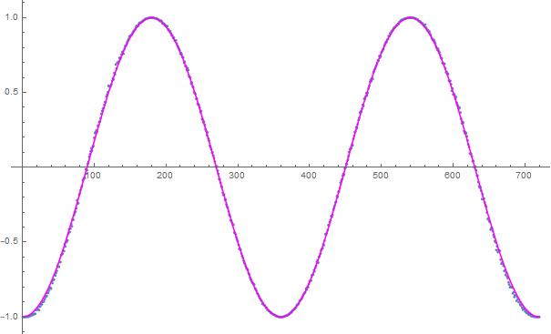
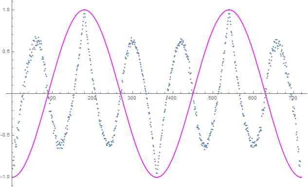
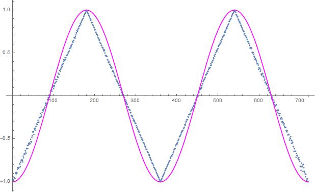
The point is that some of the curves do exceed the negative cosine in some places where both are positive. They don't lie "inside" the area enclosed by the zig-zag / saw-tooth / triangle-wave, though many people seem to think that that is what Bell's theorem says. The hidden variable is an angle.

The A and B functions: the little disks in the pictures tell you in each case what A and B are, it's the famous coloured spinning disk model, with just two colours. The A and B curves are piecewise constant. In order to make sure that there is perfect (anti) correlation at various setting differences, one is the negative of the other. Remember that Caroline Thompson had a spinning ball model with three colours, one of the colours being for "no detection". With three colours, one of the colours being "no detection", one can recover the negative cosine perfectly, as Pearle essentially showed long ago. And as Michel Fodje discovered for himself, independently. No doubt there have been others, too. Hans de Raedt (University of Groningen, Netherlands) has been publishing simulations of that nature for a long time.

Could you post your Mathematica code as a plain text file? Copy-pasting from the pdf doesn't work well. The notebook file is a text document but it contains much, much more than the Mathematica code itself. Which is hard to extract from the notebook. I'll then do a quick translation into R. It will certainly help me understand what you're doing

[gill1109]

I'm going to go ahead and post the code for this new simulation even though I am not entirely satisfied with it..., yet. Perhaps someone else might be interested in tinkering with it to improve it? Or to collaborate with it?
...
...
http://www.sciphysicsforums.com/spfbb1/EPRsims/newCS-1.pdf
http://www.sciphysicsforums.com/spfbb1/EPRsims/newCS-1.nb
It utilizes the complete states function. You can see from the code that during the constraints, the a and b vector angles subtract from themselves. I have yet to figure out a good physical justification for that. Perhaps some S^3 action at work? But the simulation is completely local and completely predictable for the A and B outcomes if you know a, b, e and lambda so it is 100 percent realistic.

The subtractions aa = (a - a) and bb = (b - b) mean that CA and CB contain values -1, 0 and +1, and these values go into AliceD and BobD too. This means that when you count joint outcomes pPP, pPN, pNP, pNN you only count the +/-1's. The claim "No Events are Dropped" is not quite true. They are not explicitly dropped. But they are not counted.

Some would say that that is correct, since physically they never happened anyway.

Michel Fodje did not have (2/Sqrt[1 + (3 \[Lambda])/\[Pi]] - 1), he had something a little bit different. But he did come amazingly close!

From a purely mathematical point of view, this is actually *exactly* Philip Pearle's (1970) model, though it is quite hard to recognise it if you would try to find it in that paper. Philip did not have that actual formula, but after you correct several misprints and some real errors (a wrong normalisation constant) in Pearle's paper, you can determine that his formula (22) (corrected) is equivalent to your (2/Sqrt[1 + (3 \[Lambda])/\[Pi]] - 1).

https://journals.aps.org/prd/abstract/10.1103/PhysRevD.2.1418 (Pearle's paper)
https://www.researchgate.net/profile/Philip_Pearle/publication/235524553_Hidden-Variable_Example_Based_upon_Data_Rejection/links/5e33616a458515072d70faeb/Hidden-Variable-Example-Based-upon-Data-Rejection.pdf

https://www.mdpi.com/1099-4300/22/1/1 (my analysis of Pearle's paper)
https://www.preprints.org/manuscript/202001.0045/v1 (my analysis of Michel Fodje's models)

I am of course proud to say here that this is the simulation model used in "Bell’s Theorem Versus Local Realism in a Quaternionic Model of Physical Space" by J. Christian https://ieeexplore.ieee.org/document/8836453

[Heinera]

The subtractions aa = (a - a) and bb = (b - b) mean that CA and CB contain values -1, 0 and +1, and these values go into AliceD and BobD too. This means that when you count joint outcomes pPP, pPN, pNP, pNN you only count the +/-1's. The claim "No Events are Dropped" is not quite true. They are not explicitly dropped. But they are not counted.

While these subtractions are indeed the culprits, the mechanism in Fred's latest attempt is not quite like you describe. The variables a and b are not detection results, but detector angles. So, if the hidden variable satisfy a certain condition the detector angle is simply set to zero. This is of course absurd, since the setting of the detectors should not depend on the value of the hidden variable.

[gill1109]

The subtractions aa = (a - a) and bb = (b - b) mean that CA and CB contain values -1, 0 and +1, and these values go into AliceD and BobD too. This means that when you count joint outcomes pPP, pPN, pNP, pNN you only count the +/-1's. The claim "No Events are Dropped" is not quite true. They are not explicitly dropped. But they are not counted.

While these subtractions are indeed the culprits, the mechanism in Fred's latest attempt is not quite like you describe. The variables a and b are not detection results, but detector angles. So, if the hidden variable satisfy a certain condition the detector angle is simply set to zero. This is of course absurd, since the setting of the detectors should not depend on the value of the hidden variable.

Thanks! You are better at reading Mathematica than I am. (I am pretty lousy at checking other people's code. Bad enough at checking my own).

[FrediFizzx]

The subtractions aa = (a - a) and bb = (b - b) mean that CA and CB contain values -1, 0 and +1, and these values go into AliceD and BobD too. This means that when you count joint outcomes pPP, pPN, pNP, pNN you only count the +/-1's. The claim "No Events are Dropped" is not quite true. They are not explicitly dropped. But they are not counted.

While these subtractions are indeed the culprits, the mechanism in Fred's latest attempt is not quite like you describe. The variables a and b are not detection results, but detector angles. So, if the hidden variable satisfy a certain condition the detector angle is simply set to zero. This is of course absurd, since the setting of the detectors should not depend on the value of the hidden variable.

Yes, that is what it looks like at first glance. And no events are dropped. What happens is all the events during the constraints are at 0 lab frame angle and average to -1. Well, at 360 degrees in the plot since I shifted everything by 2pi since theta is used as an index.

However, this might be subject to some interpretation. It is not the hidden variable that necessarily "causes" the a and b vectors to become null vectors during the constraints. It could be S^3 topological action. Of course I will need to show the math of how that works then. That is the part that I am stuck on right now. Another option to consider is that the topological action needs to be in the "then" function part and then a and b don't become null vectors.
.

[gill1109]

The subtractions aa = (a - a) and bb = (b - b) mean that CA and CB contain values -1, 0 and +1, and these values go into AliceD and BobD too. This means that when you count joint outcomes pPP, pPN, pNP, pNN you only count the +/-1's. The claim "No Events are Dropped" is not quite true. They are not explicitly dropped. But they are not counted.

While these subtractions are indeed the culprits, the mechanism in Fred's latest attempt is not quite like you describe. The variables a and b are not detection results, but detector angles. So, if the hidden variable satisfy a certain condition the detector angle is simply set to zero. This is of course absurd, since the setting of the detectors should not depend on the value of the hidden variable.

Yes, that is what it looks like at first glance. And no events are dropped. What happens is all the events during the constraints are at 0 lab frame angle and average to -1. Well, at 360 degrees in the plot since I shifted everything by 2pi since theta is used as an index.

However, this might be subject to some interpretation. It is not the hidden variable that necessarily "causes" the a and b vectors to become null vectors during the constraints. It could be S^3 topological action. Of course I will need to show the math of how that works then. That is the part that I am stuck on right now. Another option to consider is that the topological action needs to be in the "then" function part and then a and b don't become null vectors.
.

OK, so in a sense no events are dropped. They are all represented somewhere in your graph. But the events which go to make up the value of the curve at any setting difference theta not equal to zero, are only those events where the difference in the settings was theta *and* both particles were detected. Not *all* the events where the difference in settings was theta.

You performed a non local operation: if either particle is not detected then the settings of both those particles are altered and the outcomes are altered too.

[FrediFizzx]

Yes, that is what it looks like at first glance. And no events are dropped. What happens is all the events during the constraints are at 0 lab frame angle and average to -1. Well, at 360 degrees in the plot since I shifted everything by 2pi since theta is used as an index.

However, this might be subject to some interpretation. It is not the hidden variable that necessarily "causes" the a and b vectors to become null vectors during the constraints. It could be S^3 topological action. Of course I will need to show the math of how that works then. That is the part that I am stuck on right now. Another option to consider is that the topological action needs to be in the "then" function part and then a and b don't become null vectors.
.

OK, so in a sense no events are dropped. They are all represented somewhere in your graph. But the events which go to make up the value of the curve at any setting difference theta not equal to zero, are only those events where the difference in the settings was theta *and* both particles were detected. Not *all* the events where the difference in settings was theta.

You performed a non local operation: if either particle is not detected then the settings of both those particles are altered and the outcomes are altered too.

All particles are detected so not sure what you mean here. Theta ends up being 0 only if both a and b are null vectors during the constraints. But theta can also be 0 not during the constraints if a and b are equal.
.

[gill1109]

I will study the code again. I don't often use Mathematica.

By the way, I have thoroughly revised my paper about the triangle wave and the cosine curve, http://arxiv.org/abs/1312.6403

The famous singlet correlations of a composite quantum system consisting o two spatially separated components exhibit notable features of two kinds. The first kind consists of striking certainty relations: perfect correlation and perfect anti-correlation in certain settings. The second kind consists of a number of symmetries, in particular, invariance under rotation, as well as invariance under exchange of components, parity, or chirality. In this note, I investigate the class of correlation functions that can be generated by classical composite physical systems when we restrict attention to systems which reproduce the certainty relations exactly, and for which the rotational invariance of the correlation function is the manifestation of rotational. invariance of the underlying classical physics. I call such correlation functions classical EPR-B correlations. It turns out that the other three (binary) symmetries can then be obtained "for free": they are exhibited by the correlation function, and can be imposed on the underlying physics by adding an underlying randomisation level. We end up with a simple probabilistic description of all possible classical EPR-B correlations in terms of a "spinning coloured disk" model, and a research programme: describe these functions in a concise analytic way. We survey open problems, and we show that the widespread idea that "quantum correlations are more extreme than classical physics allows" is at best highly inaccurate, through giving a concrete example of a classical correlation which satisfies all the symmetries and all the certainty relations and which exceeds the quantum correlations over a whole range of settings.

The paper has a lot of pictures of possible curves which can be got by simulation! And pictures of the spinning coloured disks which produce them, too. There are lots of open problems and, no doubt, with more experiments one might make more interesting discoveries.

[FrediFizzx]

Here is one for you produced by the +/-1 outcomes during the constraints.



If you subtract that from the straight line data,



you get the negative cosine curve.


.

[gill1109]

Here is one for you produced by the +/-1 outcomes during the constraints. If you subtract that from the straight line data, you get the negative cosine curve.

Cool!

[FrediFizzx]

Here is one for you produced by the +/-1 outcomes during the constraints. If you subtract that from the straight line data, you get the negative cosine curve.

Cool!

Yeah, it is pretty cool. I wasn't expecting the data to be so organized in the first plot. It looks like some kind of polynomial cubic function. The trick is to figure out how to split it for stations A and B.
.