The 64 thousand Euro challenge

[gill1109]

What is the QM prediction for isolated separated measurements using the event by event outcomes? The correct answer would be... Ta Da! QM can't predict the event by event outcomes!
.

Fred, by “QM” do you mean just the deterministic part of QM (unitary and hence reversible evolution of vectors in Hilbert space) or do you also include Born’s rule and the non-unitary, irreversible, von Neumann- Lüders wave-function collapse?

[gill1109]

We must be clear that when it comes to atoms, language can be used only as in poetry.
Niels Bohr

Quantum mechanics makes absolutely no sense
Roger Penrose

The ‘paradox’ is only a conflict between reality and your feeling of what reality ‘ought to be’
Richard Feynman

If it is correct, it signifies the end of physics as a science
Albert Einstein

I think I can safely say that nobody understands quantum mechanics
Richard Feynman

If you are not completely confused by quantum mechanics, you do not understand it
John Wheeler
 
I do not like it, and I am sorry I ever had anything to do with it
Erwin Schrödinger

[Austin Fearnley]

I have placed a new paper online at vixra: Antiparticles and the Nature of Space. https://vixra.org/abs/2101.0179

I have used this particular forum heading just to annoy Richard. Well, no. As a guest I cannot start a new topic. I know I am not entitled to Richard's prize money as my model uses the conspiracy loophole. But IMO my paper is relevant here as I have resolved this issue to my own satisfaction.

Some history. I first wrote in this forum and its predecessor s.p.f forum to develop my preon model. Fred, at some early stage, enlisted my help on the computing side for Joy's model. Of course I was early disposed in favour of Joy's model. But there were doubts which arose in the programming, despite me quite liking the S3 model of the universe and its particles. Programming in geometric algebra was beyond me and, later, Chantal Roth rode in to the rescue. But there were loophole issues in the programming because of missing data. If the universe is S3 then if you generate data in R3 it should not be a big surprise if not all of that data are valid in S3. AFAIK the data created are still not programmed directly into S3? I mean directly into S3 space rather than created on GA software.

My previous (2020) paper says that Chantal's 'random on a sphere' generation of random data is still not appropriate for polarised particles. Who says so? I do, at least. In my particle model, if a particle is polarised in direction theta then there will be more chance that the hidden vector will point along theta than expected at random. Moreover, there is a dynamism in the particle which ensures that the measurement outcome has a statistical element to it. And in my retrocausal model, the electron is polarised when it is measured in a Bell experiment.

IMO Bell's Theorem was very important in making me look for the loophole that nature uses. Nature is even more important than Bell's Theorem and nature can use a loophole if it needs to. Nature does not break the Bell Inequalities in order to obtain the Bell correlation of - cos theta. All that is needed is antiparticles travelling backwards in time.

In Joy's model, pairs of particles are generated in GA spaces either (+,+) or (-,-). In my model, pairs of particles are generated in GA spaces either (+,-) or (-,+). A paper by James M. Chappell et al: Time As a Geometric Property of Space (2016, https://doi.org/10.3389/fphy.2016.00044 ) has time as a dependent scalar dimension within a geometric algebra description of space. I use Chappell's paper to justify particles and antiparticles travelling in different time directions.

I am hoping this is my final physics paper as my back is getting too old to sit for hours at a desktop PC editing papers. I am in the UK and am old enough to be getting the Oxford vaccine next Friday. (Unless the EU stops my jab!)

[gill1109]

I have placed a new paper online at vixra: Antiparticles and the Nature of Space. https://vixra.org/abs/2101.0179

I have used this particular forum heading just to annoy Richard. Well, no. As a guest I cannot start a new topic. I know I am not entitled to Richard's prize money as my model uses the conspiracy loophole. But IMO my paper is relevant here as I have resolved this issue to my own satisfaction.

Some history. I first wrote in this forum and its predecessor s.p.f forum to develop my preon model. Fred, at some early stage, enlisted my help on the computing side for Joy's model. Of course I was early disposed in favour of Joy's model. But there were doubts which arose in the programming, despite me quite liking the S3 model of the universe and its particles. Programming in geometric algebra was beyond me and, later, Chantal Roth rode in to the rescue. But there were loophole issues in the programming because of missing data. If the universe is S3 then if you generate data in R3 it should not be a big surprise if not all of that data are valid in S3. AFAIK the data created are still not programmed directly into S3? I mean directly into S3 space rather than created on GA software.

My previous (2020) paper says that Chantal's 'random on a sphere' generation of random data is still not appropriate for polarised particles. Who says so? I do, at least. In my particle model, if a particle is polarised in direction theta then there will be more chance that the hidden vector will point along theta than expected at random. Moreover, there is a dynamism in the particle which ensures that the measurement outcome has a statistical element to it. And in my retrocausal model, the electron is polarised when it is measured in a Bell experiment.

IMO Bell's Theorem was very important in making me look for the loophole that nature uses. Nature is even more important than Bell's Theorem and nature can use a loophole if it needs to. Nature does not break the Bell Inequalities in order to obtain the Bell correlation of - cos theta. All that is needed is antiparticles travelling backwards in time.

In Joy's model, pairs of particles are generated in GA spaces either (+,+) or (-,-). In my model, pairs of particles are generated in GA spaces either (+,-) or (-,+). A paper by James M. Chappell et al: Time As a Geometric Property of Space (2016, https://doi.org/10.3389/fphy.2016.00044 ) has time as a dependent scalar dimension within a geometric algebra description of space. I use Chappell's paper to justify particles and antiparticles travelling in different time directions.

I am hoping this is my final physics paper as my back is getting too old to sit for hours at a desktop PC editing papers. I am in the UK and am old enough to be getting the Oxford vaccine next Friday. (Unless the EU stops my jab!)

You don’t annoy me, you delight me, Austin! Retrocausality is the way to go, according to quite a few very smart people. I can see its use as a mathematical device and hence also as a way to understand physics, but if this is what you need to explain quantum phenomena, then as far as I am concerned they are beyond human understanding. Doesn’t matter. Why should everything be explainable in terms of what our naturally evolved brains will accept as an explanation? I think that Maxwell even said the same about his own theory. It is how it is.

[Austin Fearnley]

Richard

I am fairly surprised but pleased at your attitude to retrocausality. I had always assumed that your position was that the only answer was for Bell's Inequalities to be broken legitimately ie not by a loophole. Which would typically imply non-locality or non-reality or the multiverse etc.

I appear to have a different attitude to you on natural intuition on what the world is like. I obtained my viewpoint not from my own application of mathematical devices. I followed about 300 hours over ten years ago of Susskind's online physics lectures for old folks. Quite mathematical and very enjoyable. The main influence on me for this current work was the ideas in string theory relating to compactification of dimensions (and universes) and the similarity to the compactification of data outputs to binary digits. This crosses with my work on preon theory. My four preons can make all the Standard Model particles. But there are hexarks within my preons and strings are at about the level of the hexarks. So I am not too bothered that the LHC did not find strings.

I always liked Joy's S3 model of the universe and of particles. If time can be a trivector in S3 then the block universe of spacetime can be a closed spacetime object where the moibus strip effect returns space back on itself and also returns time back on itself.

I have only applied low-key maths, or even lego-like logic, in developing my models but I have tried to work to the Standard Model results which have been put together by experts.

There are some points blocking acceptance of retrocausality. More note should be taken of relativity. I see the world as local at both micro level and at macro level. Unfortunately, at macro level it seems like information is being transferred instantly from Alice's device to Bob's device (say). On the micro level, the information goes backwards in time from Alice to Oven and then forwards from Oven to Bob. Seems very local to me as could be done in a game of life using only moves to adjoining squares. Alice only records either + or - as outcomes for antiparticles. Just use all the +1s recorded by Alice (on antiparticles - note that we cannot know which are particles and antiparticles so this is only a thought experiment). Some of those antiparticles will be paired with particles measured by Bob, and they will be measured by Bob with some as + and some as -. So Bob will be passed by Alice the information: 'all these are + results'. That is also the info that Alice notes in her results book for use in the post analysis. That info does not help Bob to know which particles will be recorded by him as + and which -. The other effect of retrocausality is that all particles to be measured by Bob have been polarised along or against Alice's detector angle, which is at an angle theta to Bob's device. That is true for all those + outcomes passed by Alice, so no need to be concerned as this is not individual particle level data.

I am not an expert on anything and certainly not on S-G devices, I have read doubts being raised about it having a two stage effect. First polarising and then measuring. So all particles initially get polarised by Bob's device to Bob's polarisation angle (either along or against). Well, that is fine. The polarisation event by Bob determines how many of the particles (the ones with partners measured as + by Alice) will be passed as + by Bob. (And that also determines the number of - results.) [Malus's Law gives this number.] This number of + results is directly caused by the the fixed angle theta between measuring device polarisation angles. The actual measurement by Bob's S-G device determines which individual particles get + or - results. That measurement depends on individual particle h.v.s which are dynamic. Because they are dynamic there is a chance element to the + or - result, though the total number of + results depends only on theta.

This is too much to post here so if I have any further points I will put them on my website. Unless anyone here is interested in more.

[gill1109]

I think that retrocausality makes no sense as an explanation but if it makes interesting and falsifiable predictions, then go for it. I learn from quantum mechanics that the microscopic world cannot be understood in a way which makes sense to our instincts. One does not understand new mathematics, one gets used to it.

[Austin Fearnley]

Richard,

Feynman used Advanced and Retarded waves, backwards and forwards in time respectively. My preon model has preons and antipreons which could represent similar. I have used positrons in my retrocausal paper and did not use my preon model, but it may be interesting if I use preons here. And use photons.

The two photons have properties of spin +1 and spin-1. In my model these are made of four preons each: BBC’C’ and B’B’CC. If the electron is matter (forwards in time) then B’B’CC is also forwards in time. Eight minutes may pass for us as a photon travels from sun to earth, but the photon does not experience any passage of time. The photon will experience a curve from the sun to earth as a relativistically completely compressed line, that is a point. In its own frame, the photon starts at a point and finishes at the same point, with zero time elapsed. A neat trick?

The advanced and retarded waves may help it. The B’B’ preons are travelling backwards in time and they set out from earth to sun just as the CC preons are travelling from sun to earth. So the B’B’ preons act like pathfinders on the journey.

I think that this view can also work for superdeterminism. If you are simulating photon hidden variables then a block universe distribution of paths implies that a random sample of paths may be not accurate enough as the paths are pre-fixed. For me that implies superdeterminism is (maybe covertly?) relying on retrocausality. (However, I can’t abide the philosophy in Bell, retrocausality and superdeterministic papers, so I may be wrong wrt superdeterminism).

Another issue, that occurred in the retractionwatch debate online, was that the use of + and - trivectors was to be banned when used in one calculation. But, If the universe is using + and- trivectors simultaneously then the maths needs to follow reality rather than lead it. It gets worse!!! In our vast area of the universe we can pick say the + trivector as the direction of the overall thermodynamic arrow of time. And that direction stays unchanged and unchallenged in any calculation. This is the reason that I maintain that my model is not well described by the 'causality' in the word 'retrocausality'. Nothing challenges the macroscopic arrow of time in the macroscopic world.

But at the microscopic level? At a creation event of a particle-antiparticle pair, space must divide into two separate regions (in this model). So that is two simultaneous trivectors in my model (note - this is not the case for Joy’s model). But, worse, the photon B’B’CC is the spin -1 forwards in time photon and within it there are two time directions as B’B’ and CC which are travelling in opposite time directions. A question. Does B’B’ need its own trivector of space (a third nesting) or can it exist in the ‘wrong’ sign trivector and stay at the second level of nesting? Ie do you only get space bifurcation at particle-antiparticle creation events? A third level of trivector sign is needed as in my model there is no difference between a particle and an antiparticle except for the trivector sign of the space it is travelling in. So, to make models of preons one would need to use three levels of nested trivectors.

Those were ideas following on from my 2021 paper on space/time but my 2020 paper on Bell/ retrocausality made me review the up/ down QM descriptions. To model Bell’s Theorem using retrocausality using classical physics, which is what I did, made me revise and change my ideas of |up> and |down>. I lost my static view and replaced it with a dynamic view. After a measurement in the up/down vector, the electrons are either |up> or |down>. Only two possibilities. Previously I imagined the up electron had a multitude of different electron hidden variables within it. That is static hidden variables. But a change from static to dynamic allows me to keep the multitude of h.v.s but the dynamic picture leaves just one |up> electron so long as the dynamism includes or covers all possible static h.v.s. A dynamic view of h.v.s did not previously correspond with my view that a h.v. should be gyroscopically stable/static. However, in my preon model an electron has four preons which could maybe cause the internal instability. It was next a small step to modelling what the single statistical distribution of h.v.s in the |up> electron should be. That was straightforward using Malus’s Law and gives a statistical envelope of the h.v. directions. So there is only one |up> electron in a statistical description over a period of time. But at any instant for an |up> electron there are a myriad of potential h.v.s. So the h.v.s are say the raw data which are averaged out in a statistical picture over time. It also follows that the statistical picture of the |up> or polarised electron determines the overall probability of its measurement outcome whereas the actual h.v. Is needed to provide the actual individual outcome.

There is a randomness in the measurement outcome even if the h.v. Is known. Because of the dynamism, to predict the outcome you need to know the h.v. vector AND also where that vector is at the instant of measurement. The h.v. Is not a fixed vector in space, it is more like a vector from the centre of earth to say Oxford. It is fixed only in the sense that Oxford is fixed, but the Oxford vector is dynamic over time as the planet rotates. So knowing the electron h.v. Is insufficient to predict a measurement outcome as the outcome also depends on time.

[gill1109]

Richard,

Feynman used Advanced and Retarded waves, backwards and forwards in time respectively. My preon model has preons and antipreons which could represent similar. I have used positrons in my retrocausal paper and did not use my preon model, but it may be interesting if I use preons here. And use photons.

The two photons have properties of spin +1 and spin-1. In my model these are made of four preons each: BBC’C’ and B’B’CC. If the electron is matter (forwards in time) then B’B’CC is also forwards in time. Eight minutes may pass for us as a photon travels from sun to earth, but the photon does not experience any passage of time. The photon will experience a curve from the sun to earth as a relativistically completely compressed line, that is a point. In its own frame, the photon starts at a point and finishes at the same point, with zero time elapsed. A neat trick?

The advanced and retarded waves may help it. The B’B’ preons are travelling backwards in time and they set out from earth to sun just as the CC preons are travelling from sun to earth. So the B’B’ preons act like pathfinders on the journey.

I think that this view can also work for superdeterminism. If you are simulating photon hidden variables then a block universe distribution of paths implies that a random sample of paths may be not accurate enough as the paths are pre-fixed. For me that implies superdeterminism is (maybe covertly?) relying on retrocausality. (However, I can’t abide the philosophy in Bell, retrocausality and superdeterministic papers, so I may be wrong wrt superdeterminism).

Another issue, that occurred in the retractionwatch debate online, was that the use of + and - trivectors was to be banned when used in one calculation. But, If the universe is using + and- trivectors simultaneously then the maths needs to follow reality rather than lead it. It gets worse!!! In our vast area of the universe we can pick say the + trivector as the direction of the overall thermodynamic arrow of time. And that direction stays unchanged and unchallenged in any calculation. This is the reason that I maintain that my model is not well described by the 'causality' in the word 'retrocausality'. Nothing challenges the macroscopic arrow of time in the macroscopic world.

But at the microscopic level? At a creation event of a particle-antiparticle pair, space must divide into two separate regions (in this model). So that is two simultaneous trivectors in my model (note - this is not the case for Joy’s model). But, worse, the photon B’B’CC is the spin -1 forwards in time photon and within it there are two time directions as B’B’ and CC which are travelling in opposite time directions. A question. Does B’B’ need its own trivector of space (a third nesting) or can it exist in the ‘wrong’ sign trivector and stay at the second level of nesting? Ie do you only get space bifurcation at particle-antiparticle creation events? A third level of trivector sign is needed as in my model there is no difference between a particle and an antiparticle except for the trivector sign of the space it is travelling in. So, to make models of preons one would need to use three levels of nested trivectors.

Those were ideas following on from my 2021 paper on space/time but my 2020 paper on Bell/ retrocausality made me review the up/ down QM descriptions. To model Bell’s Theorem using retrocausality using classical physics, which is what I did, made me revise and change my ideas of |up> and |down>. I lost my static view and replaced it with a dynamic view. After a measurement in the up/down vector, the electrons are either |up> or |down>. Only two possibilities. Previously I imagined the up electron had a multitude of different electron hidden variables within it. That is static hidden variables. But a change from static to dynamic allows me to keep the multitude of h.v.s but the dynamic picture leaves just one |up> electron so long as the dynamism includes or covers all possible static h.v.s. A dynamic view of h.v.s did not previously correspond with my view that a h.v. should be gyroscopically stable/static. However, in my preon model an electron has four preons which could maybe cause the internal instability. It was next a small step to modelling what the single statistical distribution of h.v.s in the |up> electron should be. That was straightforward using Malus’s Law and gives a statistical envelope of the h.v. directions. So there is only one |up> electron in a statistical description over a period of time. But at any instant for an |up> electron there are a myriad of potential h.v.s. So the h.v.s are say the raw data which are averaged out in a statistical picture over time. It also follows that the statistical picture of the |up> or polarised electron determines the overall probability of its measurement outcome whereas the actual h.v. Is needed to provide the actual individual outcome.

There is a randomness in the measurement outcome even if the h.v. Is known. Because of the dynamism, to predict the outcome you need to know the h.v. vector AND also where that vector is at the instant of measurement. The h.v. Is not a fixed vector in space, it is more like a vector from the centre of earth to say Oxford. It is fixed only in the sense that Oxford is fixed, but the Oxford vector is dynamic over time as the planet rotates. So knowing the electron h.v. Is insufficient to predict a measurement outcome as the outcome also depends on time.

There's a lot of physics I don't know about. But this is what I say to people with your point of view.

Please think of a loophole-free Bell experiment, using the singlet state of two spin-half particles, in which the setting choice (0 or pi/2 on Alice's side, pi/4 or 3 pi/4 on Bob's side) is made not by human free will, or by tossing coins, but by preparing spin-half particles in the spin up (z -direction) state, and then measuring them in the x-direction. Thus we have a pure state of four spin-half particles all being measured, resulting in four binary outcomes.

Please do the calculations using your retrocausal ideas and show us how the causality generates the measurement setting choices from the measurement outcomes.

I ask both retrocausal and superdeterminism people to work out this little example for me. They always refuse to do it. I think such people are scared of what they will see. They haven't assimilated what Bell's theorem means to their fancy math physics.

If your approach has got Born's law and if it reproduces conventional QM results there should be no problem. But otherwise, you will see that it is just a mathematical trick which does not explain anything, in the sense it does not help us understand what actually goes on; it's just some algebra which gives the right answer by some kind of magic. One can get used to the algebra, one can even develop feeling, intuition, for it, but that doesn't mean you *understand* reality better. You can *predict* it better. In some sense, you have *explained* a bit of physical reality. Probably, one cannot hope for more. This was already said more than a century ago about Maxwell's theory.

I think that whatever way you look at it, it will all come down to quantum magic in the end. You can dress it up in sophisticated maths which almost nobody understands, but you are just a present-day high-priest or shaman. [Such people often have immense knowledge and fantastic skills]. But, really, it's just another religion. Human beings need religion, it's built into our "software" (are brains are pretty soft things) by evolution. We need high priests and shamans.

[Austin Fearnley]

Richard wrote:

Please think of a loophole-free Bell experiment, using the singlet state of two spin-half particles, in which the setting choice (0 or pi/2 on Alice's side, pi/4 or 3 pi/4 on Bob's side) is made not by human free will, or by tossing coins, but by preparing spin-half particles in the spin up (z -direction) state, and then measuring them in the x-direction. Thus we have a pure state of four spin-half particles all being measured, resulting in four binary outcomes.

Hi Richard, I am just an amateur and cannot really represent retrocausalists and, definitely not, superdeterminists. As I said, I hate reading their philosophical papers. If you help me understand the task I will try (or at least think about it!).

"Please think of a loophole-free Bell experiment,"

But retrocausality is, in your terms, a loophole method ... so how can I prepare a loophole-free expt? Are you asking me to throw away retrocausality and start again using a forwards-in-time method? If so, I cannot do that as I have already IMO found the retro solution to be correct. (Note that I am not competing for prize money.)

I find the rest of the task hard to fathom. Especially, what is the point of it when IMO the retrocausal method works whatever the settings. Change any setting as often as you like, to whatever you like, even at any time within flight.

Task:
Measure electron #1 in up (+z) direction. Outcome is either + or - in +z direction.
Then re-measure it in x direction. Outcome is either + or - in x direction.
Use this outcome to choose between Alice's 0 or pi/2 setting.

Can use a similar procedure on all four electrons.
That gives you four detector settings though I am lost as to why you would want to do this... seems irrelevant to me. In a retrocausal experiment the actual settings are irrelevant to the answer, only the difference in angles between Bob's and Alice's detector, for each individual pair of particles measured, is relevant.

I have used four electrons for this task, but in the actual expt there would need to be both electrons and positrons used to make the retrocausality work.

What next?

[Austin Fearnley]

Follow up comment:
I can write a computer program to generate such random numbers, in sets of four numbers, to be used as detector settings. I will use my 'classical' electron structure to do that task. It would be just as easy to use computer generated random numbers. I will have to include a use of computer-generated random numbers anyway to faithfully use my electron structure. In the 1970s I used Fisher and Yates to generate random samples of students. I left that book in the office when I retired, but I still have my own copy of the Biometrika book of Statistical Tables, which has random numbers if I remember correctly. Still, I don't want to look up and transcribe hundreds of random numbers.

I appreciate that you think it is important to operate that way of randomising device settings, and I want to show my method works however it is constrained. But I do think there is a lot of hype around setting angles. I saw a Horizon TV program where they were using light polarisation from early formed galaxies to choose settings. To my mind that was just a waste of programme time and telescope time.

Also, at the time of measurement in my model, the positron is not yet entangled with the electron. So much for the 'spooky' entanglement. The last phase of any project is praise and glory for the non-participants, that seems to fit 'entanglement' which was not even present at the critical moment. Well that is a little unfair as the electron was entangled with the positron but only after the positron had been measured. That is, at the Oven. Actually, in my model, the electron only becomes entangled at the instant it leaves the oven. And at that very instant the (backwards-in-time) positron ceases to exist. And at the Oven, the positron passed to the electron a polarisation angle and h.v. that it did not have when it presented itself before its own measurement.

[gill1109]

Richard wrote:

Please think of a loophole-free Bell experiment, using the singlet state of two spin-half particles, in which the setting choice (0 or pi/2 on Alice's side, pi/4 or 3 pi/4 on Bob's side) is made not by human free will, or by tossing coins, but by preparing spin-half particles in the spin up (z -direction) state, and then measuring them in the x-direction. Thus we have a pure state of four spin-half particles all being measured, resulting in four binary outcomes.

Hi Richard, I am just an amateur and cannot really represent retrocausalists and, definitely not, superdeterminists. As I said, I hate reading their philosophical papers. If you help me understand the task I will try (or at least think about it!).

"Please think of a loophole-free Bell experiment,"

But retrocausality is, in your terms, a loophole method ... so how can I prepare a loophole-free expt? Are you asking me to throw away retrocausality and start again using a forwards-in-time method? If so, I cannot do that as I have already IMO found the retro solution to be correct. (Note that I am not competing for prize money.)

I find the rest of the task hard to fathom. Especially, what is the point of it when IMO the retrocausal method works whatever the settings. Change any setting as often as you like, to whatever you like, even at any time within flight.

Task:
Measure electron #1 in up (+z) direction. Outcome is either + or - in +z direction.
Then re-measure it in x direction. Outcome is either + or - in x direction.
Use this outcome to choose between Alice's 0 or pi/2 setting.

Can use a similar procedure on all four electrons.
That gives you four detector settings though I am lost as to why you would want to do this... seems irrelevant to me. In a retrocausal experiment the actual settings are irrelevant to the answer, only the difference in angles between Bob's and Alice's detector, for each individual pair of particles measured, is relevant.

I have used four electrons for this task, but in the actual expt there would need to be both electrons and positrons used to make the retrocausality work.

What next?

Don’t try to fathom anything. Don’t consult quantum philosophers. Don’t ask “why those angles”. Just tell us how your model deals with the situation which I describe here:

Measure electron #1 in up (+z) direction. Outcome is either + or - in +z direction.
Then re-measure it in x direction. Outcome is either + or - in x direction.

Use this outcome to choose between Alice's 0 or pi/2 setting for measuring electron #2.

Measure electron #4 in up (+z) direction. Outcome is either + or - in +z direction.
Then re-measure it in x direction. Outcome is either + or - in x direction.

Use this outcome to choose between Bob’s pi/4 or 3 pi/4 setting for measuring electron #3.

Show us your model. I hope it will correctly reproduce the statistics of Bell-CHSH experiments on the singlet state.

I want to understand *your* model. Because of Bell’s theorem (a piece of trivial mathematics, not philosophy or religion) your modelling of this situation must entail that the measurement outcomes of electrons 1 and 4 are somehow determined, knowing the outcomes of 2 and 3. It cannot satisfy ‘no-conspiracy’.

Alternatively, it must be non-local, or non-realist.

Either way, it should give the right answer by just “shutting up and calculating” but not, I think, resolve any mystery. It won’t tell us “what is really going on”. It will be just mathematical trickery. Or it will be wrong. It should be an easy exercise. If you need to introduce further particles moving backward in time, feel free.

[Austin Fearnley]

Hi Richard

I am a guest here and cannot start a new thread. Maybe you or Fred should start a new thread on 'Bell and retrocausality'? As I wrote before, I know that I do not qualify for your prize money as my method does not defeat Bell's Inequalities but simply bypasses them via retrocausality using your conspiracy loophole. But my method does reproduce the -cos theta correlation.

Richard wrote:
Don’t try to fathom anything.

I am trying to close down my physics work as I am feeling too old now and I have the feeling that what you are suggesting will involve me in a lot of computer programming work. I am prepared to do the work if it is meaningful. I don't know if it is meaningful unless I fathom why you are asking. I do not want to input a lot of effort if at the end you again simply say that you do not like the method. Shut-up-and-calculate is for working according to QM. Shut-up-and-calculate is not for following the rules of Richard Gill [no offense intended though :)]

I have already in the appendix of my June 2020 vixra paper https://vixra.org/abs/2101.0179 given my computer code for using my model to give Malus Law results in a particle-at-a-time simulation. In the main body of that paper I describe my classical model of the electron and the photon and show how that model can be used to give - cos theta for the Bell correlation as long as the antiparticles are travelling backwards in time.

I completely accept that I cannot get -0.707 for a forwards in time Bell correlation for the detector settings of 0 deg for Alice and 45 deg for Bob. I have never bothered with simulating a CHSH design set up as I believe it is a waste of time in a simulation. I have normally used a single setting for each detector of Alice and Bob.

However it is easy for me to describe in words what you are asking, despite me believing it is completely an over-the-top exercise. If I cannot get a result for a simulation using 0 and 45 deg then why further complicate matters.

Anyway:

Richard wrote:
Measure electron #1 in up (+z) direction. Outcome is either + or - in +z direction.
Then re-measure it in x direction. Outcome is either + or - in x direction.

Use this outcome to choose between Alice's 0 or pi/2 setting for measuring electron #2.

The first step is the most complicated as the incoming electron#1 has to be assumed to be unpolarised as I have no history for it of previous measurements.
Generate a random number between 0 and 1 and multiply it by 2pi to give 'angle1'.
That gives a simulated polarisation angle in the xz plane. 'up' corresponds to 'angle1' = 0 ie along the z axis.

Given a host of such electrons with polarisation angle = angle1, the average number of electrons measured in the up direction is (using Malus's Law) proportional to cos^2 theta where theta = angle1-zero deg, ie theta equals angle1.

Of course, since electron#1 is in general unpolarised its average value of angle1 will be a random value and so 50 per cent of all electrons will be polarised 'up'.

But to get a measurement for an individual electron#1, knowing the polarisation is 'angle1' when measured, is not enough to know what the measurement outcome will be. We need a second level of random input of the hidden variable value.

QM measurements tell us that when an individual electron is measured as 'up' then if it is measured again and again in the 'up' direction it will still be recorded as 'up'. This means that the hidden variables of an 'up' electron [which are responsible for the measurement outcome] are all pointing within 90 degrees of 'up'. My model has these h.v. angles as dynamic but fitting within a statistical envelope calculated using Malus's Law.

Next measure electron#1, with polarisation angle = angle1, in the up direction. That is along the z axis in the xz plane. All the h.v.s in electron#1 must be pointing in the direction angle1 plus or minus 90deg. (so that repeated measurements in the angle1 polarisation setting would not change any measurement results in repeated measurements along angle1.)

Further, these h.v.s have to conform to a distribution set by Malus's Law. Basiclly more h.v.s need to point at angle1 than not. The distribution is NOT random (which is why random on a sphere simulation methods do not work).

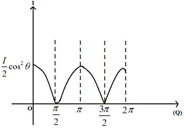
Next a little calculus. Malus's Law for electrons gives a cumulative result. Ranging from 'all pass' at theta = zero deg (difference in settings of first and second filters) to 'half shall pass' at theta = 90 deg. These are cos^2 zero/2 deg and cos^2 90/2 deg resp. The divisor of '2' is used to switch from the normal law for photons to an adapted law for electrons.

But for the statistical envelope of h.v.s about angle1 we need a density function rather than the cumulative density function given by Malus's Law. To get the density function we just differentiate.
But first, I want the distribution to run from 0 to 180 deg not from -90 to +90 deg, see EXTRACT below, so I need to differentiate
1 - cos^2 (theta/2), rather than cos^2 (theta/2). This gives 0.5*sin theta for the statistical envelope where theta runs from 0 to 180 deg.

This function yields 0 at theta = 0 and 180 deg and yields 0.5 at theta = 90. Total density = 1 over the whole curve or envelope. This shows that no h.v.s point at 90 deg away from the polarisation angle of an electron while most point along the polarisation angle.

Next pick an individual h.v. at random in this curve at the instant of measurement. My electron structure is dynamic but if I pick the instant of measurement than it is a static vector.


[ABC] Next, I choose a random number between 0 and 1 to help determine a h.v.
at the instant of measurement.

Need to switch back to the cumulative density functon for this step. (It was useful to obtain the density function to see how the h.v.s are distributed about the polarisation angle, but sorry its back to the cumulative density function.) Let the random number represent the cumulative number of h.v.s in the statistical envelope starting at theta=0. [Now see Extract#2 below for more details, if that helps.]

If we integrate the electron spin vector density 0.5 * sin x between x = 0 and x = psi, we get 0.5(-cos psi - -cos(0)).
= -0.5 * cos psi +0.5.

Set this integral to be p, the random cumulative probability for the generated electron.

So p = -0.5 * cos psi +0.5
and hence cos psi = 1-2p.

and psi is the angle whose cosine is 1-2p. Which is arccos(1-2p).

So now we have an electron with a known spin vector at angle psi. If this angle is greater [this should read 'less'] than the angle between the electron polarisation angle and the measuring angle (0 degrees for the first measurement along the z axis) then the particle passes the filter as +1.
This is where the two polarisation angles are separated by between 0 and 180 deg. If that angle is greater than 180 deg then we need to use -up as the electron polarisation angle and start again.

So, after all that, we have finished stage 1 of preparing one detector setting.

Next, we re-measure in direction +x axis. As this is a 90 deg difference in polarisation angles we know that 50 per cent of electrons will pass the filter, on average. But what about our particular electron#1?

We need to go back to instructions at [ABC] above and work it through. To summarise, we end up with another angle for the h.v. as phi' =
arccos(1-2p') where phi' and p' are new values. If phi' is less than 90 deg then measurement = +1.


Measurement +1 refers to Alice getting setting 0 deg rather than pi/2.

Note that I have not used retrocausality yet as all this calculation was necessary just to program a particle-at-a-time method for Malus's Law used in a forwards-in-time method.

EXTRACT#1 from appendix of my june 2020 vixra paper:
'
' To find the distribution of individual spin vectors (at angles of phi) is is necessary to differentiate not
' cos squared (phi/2)
' but 1 - cos squared (phi/2),
' and 1 - cos squared (phi/2) = 0.5 - 0.5 * cos phi
' which differentiates to 0.5 sin phi.
' This is the curve which is plotted for electrons in Figure A of the report: "Malus's Law and Bell's Theorem with local hidden variables".

EXTRACT#2 from appendix of my june 2020 vixra paper:
' First, by generating a random number between 0 and 1 to represent a random cumulative probability of a particle
' lying on the spin vector distribution curve. Next, we need to find out what the spin vector angle (psi) is, for the
' generated particle, corresponding to that random cumulative probability (p).
'
' If we integrate the electron spin vector density 0.5 * sin x between x = 0 and x = psi, we get 0.5(-cos psi - -cos(0)).
' = -0.5 * cos psi +0.5.
'
' Set this integral to be p, the random cumulative probability for the generated electron.
'
' So p = -0.5 * cos psi +0.5
' and hence cos psi = 1-2p.
'
' and psi is the angle whose cosine is 1-2p.
'
' That is commonly called arccos(1-2p)
'
' But in MS visual basic the arccos function does not exist and so the function used is a convoluted, but standard,
' combination of arctan functions.
'
' So now we have a particle with a known spin vector angle psi. If this angle is greater than theta then the particle
' passes the filter, where theta is the angle between the incoming polarisation vector and the filter spin vector axis.

[Austin Fearnley]

As I wrote, I am getting too old for this lark, so I had a break! BTW I had my first covid vaccine eight days ago. My wife had the Pfizer vaccine four weeks go and had no reaction. I had the Oxford-AstraZeneca version and had mild flu symptoms for three days afterwards. Bad enough for me to want to go to bed, but not too bad really.

I believe I have explained previously/above how to use electron measurements (for my electron model) to randomly choose Alice's and Bob's detector settings. This can be done before measuring a pair of particles. The settings can be randomised repeatedly before any new pair is measured.

I would be just as happy with no randomisation. Or just use the computer's random number generator to pick random settings of detectors before every pair is measured.

My June 2020 paper at https://vixra.org/abs/2101.0179 gives, in its Appendix, computer code for my model to find Malus's Law results particle-at-a-time. I have seen it written that Malus's Law is important wrt Bell's Theorem. Gordon has written similarly in this Forum. Others dismiss Malus's Law as irrelevant. I hold that Malus's Law is extremely important wrt a Bell experiment, but only in a retrocausal interpretation of the physics underlying a Bell experiment. I have written code for my model to apply to Bell forwards-in-time but it does not even get as high a correlation as 0.5. I tried a few scenarios and I remember getting 0.396 fairly regularly for the correlation. One million pairs each time. That is because my electron model has that extra element of randomness compared to a static h.v. vector.

A forwards-in-time Bell experiment starts at the O(ven) which generates pairs of entangled particles (a pair comprises one particle plus its antiparticle). Alice and Bob measure one item from each pair. They cannot distinguish particles from antiparticles. In a simulation, some model for h.v.s is applied in order to make the measurements. Measurement outcomes are obtained, and after all measurements are obtained a 2x2 table of results is made. This table of results has a correlation of -cos theta if the Bell correlation is obtained and a significantly smaller correlation (in absolute magnitude) if the model fails.

My model for h.v.s gives about -0.396 (and certainly not -0.707) for this forwards-in-time simulation for theta = 45 deg. But that all changes when the antiparticle moves backwards-in-time.

In the retrocausal model for a Bell experiment, the experiment starts not at the O(ven) but starts with incoming positrons coming from the outer environment. Alice gets and measures approximately half of these and Bob gets and measures the other half. Say half a million each for Alice and Bob in a simulation.

Next a description of a forwards-in-time Malus experiment.
Take two polarised sunglasses. Let light pass through both sunglasses one after the other. Rotate one of the sunglasses and watch the light transmitted vary according to the degree of rotation. The amount of light passing through both sunglasses varies according to Malus's Law. (See: https://cdn1.byjus.com/wp-content/uploa ... us-law.png )

Let the first pair of sunglasses represent the measurement of Alice on her first antiparticle. The antiparticle is transmitted to the Oven, carrying the polarisation angle of Alice's detector, either for or against (+ or -). The Oven is like a black box for producing entangled pairs, and this is also the case in the forwards-in-time experiment. After the Oven, the forwards-in-time entangled electron is transmitted to Bob. Bob measures this partner electron and that represents the second pair of sunglasses in a Malus's Law experiment. The Oven has replaced a backwards-in-time positron by an exactly equivalent (hence 'entangled') forwards-in-time electron. The probability of the electron 'passing' Bob's filter is given by Malus's Law which depends only on the angle between the two detector settings. It does not matter that the settings have been randomised as the electron's entanglement means that it carries the polarisation angle from Alice's measurement into Bob's detector. Bob's detector carries Bob's random setting. Randomness of detector settings is irrelevant. Before Bob measures, the electron has polarisation along or against Alice's setting and, after Bob measures, the electron has polarisation angle along or against Bob's setting. The angle between the settings determines the probability of Bob's measurement outcome.

My June 2020 paper shows how to combine these measurements into a - cos theta correlation result. It was so obvious to me that my retrocausal method worked that I only programmed the particle-at-a-time Malus experiment and did not bother with a computer program for the retrocausal Bell experiment.

At a later point I thought that I had better check if my model could actually work forwards-in-time. So I wrote that code but only obtained 0.396 rather than 0.707.

The backwards-in-time causality means that (using the positron's time frame) Alice's positron has unknown polarisation before she measures it, as it is coming in from somewhere in the universe. After Alice's measurement the positron has a polarisation vector along or against Alice's random setting. When the positron reaches the Oven it still has the polarisation angle from Alice's setting. After the Oven, the positron is replaced by an entangled electron still with the polarisation angle from Alice's setting, but travelling forwards-in-time to Bob's device. So retrocausality is essential, as is Malus's Law. Malus's Law on its own is not enough.

[Austin Fearnley]

I believe that my description is complete. It is not a computer program but describes a program that could be written, and a Bell's experiment program with randomised S-G settings before each measurement. If that is not believable enough then I will write one in June 2021 after I have had another break.

IMO I have already written a good enough program in the appendix of my June 2020 vixra paper https://vixra.org/pdf/2006.0160v1.pdf Malus’s Law and Bell’s Theorem with local hidden variables.

If one does not like backwards-in-time motion of antiparticles then so be it. But it must be completely evident that backwards-in-time antiparticles in a Bell experiment give exactly the same results as a normal forward-in-time Malus's Law experiment. Further, the antiparticles leave Alice's S-G and head back to the source with polarisation vectors along or against Alices S-G polarisation vector. The electrons therefore (using conservation of angular momentum) leave the source as entangled particles and head (forwards-in-time) to Bob's S-G having polarisation angles either along or against Alice's S-G's polarisation vector. That guarantees a Malus's Law result agreeing with a Bell correlation.

There is no need to bother about randomised settings as the setting angle is carried backwards-in-time by the positron and then passed to the entangled electron whatever the setting angle is.

My electron and photon are classical objects.
My 2020 program can be used to simulate S-G measurement outcomes using classical particle structures.
My particle structure is in two parts.
First, the polarisation angle. After a measurement in the |up> direction the electron is either polarised along or against the 'up' direction, so it is
(1)
(0)

or

(0)
(1)

There are no other alternatives. Just two states, and the 'up' state is identical for all 'up' electrons, and in that sense the description is complete.

But that is 'complete' in a statistical sense as IMO that 'up' state is dynamic and contains within it a host of h.v. directions, and it is the hidden variable vector direction at the instant of measurement that determines the measurement outcome. So, is the h.v. that causes the outcome the true h.v. of that up electron? NO. The one and only up electron is dynamic and cycles through all those h.v. directions and it is just chance which h.v. direction is the one causing the outcome. There is just one h.v. vector at any instant, but over a period of time the h.v. cycles through a whole range or allowed envelope of directions. That envelope has a statistical curve to describe it. I do not know why it is not (in 2D anyhow) simply the Normal curve, but it is instead the 0.5 sin (alpha) curve with a maximum of 0.5 pointing in the direction of the polarisation angle (at alpha = 90 deg). This curve locks results into agreement with Malus's Law.

So it is true IMO that an 'up' electron has h.v.s but a single electron does not have a single unique h.v. direction at all times. The actual h.v. used for the measurement is to some extent random and depends on the instant of measurement and also depends on the constraints of the statistical envelope, and any h.v. in that envelope could be used, subject to these constraints.

That leaves entanglement as merely the conservation of angular momentum. A spooky version of entanglement may be demonstrated in other experiments and I cannot comment on those as I know nothing of them. But I hope the future of computing is not depending on the Bell version of spooky entanglement.

[gill1109]

I believe that my description is complete. It is not a computer program but describes a program that could be written, and a Bell's experiment program with randomised S-G settings before each measurement. If that is not believable enough then I will write one in June 2021 after I have had another break.

IMO I have already written a good enough program in the appendix of my June 2020 vixra paper https://vixra.org/pdf/2006.0160v1.pdf Malus’s Law and Bell’s Theorem with local hidden variables.

If one does not like backwards-in-time motion of antiparticles then so be it. But it must be completely evident that backwards-in-time antiparticles in a Bell experiment give exactly the same results as a normal forward-in-time Malus's Law experiment. Further, the antiparticles leave Alice's S-G and head back to the source with polarisation vectors along or against Alices S-G polarisation vector. The electrons therefore (using conservation of angular momentum) leave the source as entangled particles and head (forwards-in-time) to Bob's S-G having polarisation angles either along or against Alice's S-G's polarisation vector. That guarantees a Malus's Law result agreeing with a Bell correlation.

There is no need to bother about randomised settings as the setting angle is carried backwards-in-time by the positron and then passed to the entangled electron whatever the setting angle is.

My electron and photon are classical objects.
My 2020 program can be used to simulate S-G measurement outcomes using classical particle structures.
My particle structure is in two parts.
First, the polarisation angle. After a measurement in the |up> direction the electron is either polarised along or against the 'up' direction, so it is
(1)
(0)

or

(0)
(1)

There are no other alternatives. Just two states, and the 'up' state is identical for all 'up' electrons, and in that sense the description is complete.

But that is 'complete' in a statistical sense as IMO that 'up' state is dynamic and contains within it a host of h.v. directions, and it is the hidden variable vector direction at the instant of measurement that determines the measurement outcome. So, is the h.v. that causes the outcome the true h.v. of that up electron? NO. The one and only up electron is dynamic and cycles through all those h.v. directions and it is just chance which h.v. direction is the one causing the outcome. There is just one h.v. vector at any instant, but over a period of time the h.v. cycles through a whole range or allowed envelope of directions. That envelope has a statistical curve to describe it. I do not know why it is not (in 2D anyhow) simply the Normal curve, but it is instead the 0.5 sin (alpha) curve with a maximum of 0.5 pointing in the direction of the polarisation angle (at alpha = 90 deg). This curve locks results into agreement with Malus's Law.

So it is true IMO that an 'up' electron has h.v.s but a single electron does not have a single unique h.v. direction at all times. The actual h.v. used for the measurement is to some extent random and depends on the instant of measurement and also depends on the constraints of the statistical envelope, and any h.v. in that envelope could be used, subject to these constraints.

That leaves entanglement as merely the conservation of angular momentum. A spooky version of entanglement may be demonstrated in other experiments and I cannot comment on those as I know nothing of them. But I hope the future of computing is not depending on the Bell version of spooky entanglement.

Someone who is happy with backwards-in-time causation is easily pleased! I don't think that it *explains* anything; in fact, I would say that does not *explain* anything, because it obviously explains everything.

Anything that happens - then I can say, it was going to happen anyway! No need for physicists.

[Austin Fearnley]

Hi Richard

Backwards-in-time positrons give the only explanation of Bell's experimental results of -cos Θ that satisfies me.

Feynman and Wheeler started this off with advanced and retarded waves. And the use of a whole path approach using Least Action.

My solution is not a retrocausal free for all. In the macroscopic world the thermodynamic arrow of time dominates. Even in the microscopic world, particles are travelling forwards in time only. Most stuff in our environment is made of particles. Only antiparticles travel backwards in time (always). Further nothing travels forwards in time and then reverses in time. It is not so easy to manipulate the macroscopic world with this method as you claim. Further I have a paper linking antiparticles to negative mass and that can explain DM and DE. Negative mass stops the gravitational accumulation of macro bodies so there cannot be macro masses of antiparticles to play havoc with our past world. I cannot think of a way to use the antparticles to go back and change history. Though maybe it is possible in a small way? (Isn't this do-able by quantum eraser methods? Of which I know very little.)

" ...explains everything"? That is the goal of physicists. Some (most?) physicists believe there is no free will. Everything is deterministic and settled from the initial boundary conditions. In my method one would have to say that initial and final conditions of creation/annihilation settle everything 50/50 each.

[gill1109]

Hi Richard

Backwards-in-time positrons give the only explanation of Bell's experimental results of -cos Θ that satisfies me.

Feynman and Wheeler started this off with advanced and retarded waves. And the use of a whole path approach using Least Action.

My solution is not a retrocausal free for all. In the macroscopic world the thermodynamic arrow of time dominates. Even in the microscopic world, particles are travelling forwards in time only. Most stuff in our environment is made of particles. Only antiparticles travel backwards in time (always). Further nothing travels forwards in time and then reverses in time. It is not so easy to manipulate the macroscopic world with this method as you claim. Further I have a paper linking antiparticles to negative mass and that can explain DM and DE. Negative mass stops the gravitational accumulation of macro bodies so there cannot be macro masses of antiparticles to play havoc with our past world. I cannot think of a way to use the antparticles to go back and change history. Though maybe it is possible in a small way? (Isn't this do-able by quantum eraser methods? Of which I know very little.)

" ...explains everything"? That is the goal of physicists. Some (most?) physicists believe there is no free will. Everything is deterministic and settled from the initial boundary conditions. In my method one would have to say that initial and final conditions of creation/annihilation settle everything 50/50 each.

The goal of physics is to explain everything. One explanation is that everything was created 4000 years ago by an omnipotent God. Who put fossils in the ground in order to test our faith. So: some explanations are preferred to others. Explanations which lead to testable predictions are preferred. Feynman and Wheeler found novel ways to do calculations in an existing theory, an existing framework. Feynman himself emphasised that you can’t understand quantum mechanics. Colourful imagery might help you feel comfortable with tricky maths. And if your skills sort out DE and DM that’s great!

So do the backwards in time positrons cause Alice and Bob’s setting choices? One of the three has to go: locality, realism, no-conspiracy.

[Austin Fearnley]

Hi Richard

Richard wrote:
"So do the backwards in time positrons cause Alice and Bob’s setting choices? One of the three has to go: locality, realism, no-conspiracy."

I still agree with you that 'no-conspiracy' appears to be broken by my method. But there is no conspiracy at the macro level, only at the micro level. The backwards in time positrons meet whatever settings have been chosen and the method gives the Bell correlation whatever settings are chosen. Pick any settings and the method still works. It works because the backwards-in-time positron measurement setting is imposed (via entanglement) to become the electron's polarisation vector and Malus's Law does the rest. I agree that this 'seems' like a conspiracy, but there is no need for the positrons to affect the settings. I do not know why you think this is the case?

There is one issue that you raised a while ago that is interesting. My electron structure has two levels: polarisation angle (static - an average value over time of the hidden variable) and the hidden variable vector (which is dynamic over time). There is only one hidden variable for all electrons with a given polarisation vector. The dynamic h.v. gives a random element to the measurement outcome. At some stage you wrote that the random element (say using an aggregate of n coin throws) still needs to conform to deterministic outcomes. I am not sure about this. 'Yes' if the universe is completely deterministic, and that also removes free will, and gives a static, fixed, block universe.

You could cover all possible outcomes each with a different universe (the multiverse - yuk!). Or let the universe NOT be completely deterministic. Maybe a completely deterministic universe is just physicists' hubris? It is clear that the measurement outcome does need to be calculable, but is the outcome inevitable/pre-ordained/post-ordained despite the random element? Anyway, my method shows how to do that calculation.

I still have not given up on 'free will'.

That seems to me like a good place to close. I can try to forget about Bell, particles and antiparticles and physics ... unless you have more points ...

[gill1109]

Let's leave it there for the time being. I believe you haven't yet digested Bell's theorem.

I think you would like Gerard 't Hooft's book. https://link.springer.com/book/10.1007/978-3-319-41285-6. "The Cellular Automaton Interpretation of Quantum Mechanics". You may download the pdf for free.

[Austin Fearnley]

Let's leave it there for the time being.

That is fine. Where we disagree we can agree to disagree.

I believe you haven't yet digested Bell's theorem.

As Andy Capp said: "but I never tried ..."
Maybe I became involved in the theorem discussions a long time ago on this forum, but I soon agreed in general with Bell's Theorem and distilled its essence (IMO) into the impossiblilty of using forwards-in-time hidden variables with static vectors to obtain a simulation of the Bell correlation for alpha=0 deg and beta=45 deg in R^3. I spent my time trying to get a simulation which worked to my own satisfaction. It needed some randomness in the measurement outcomes and retrocausality for the positron. It was never my intention to understand the full frills of Bell's Theorem as it is a no-go theorem. My focus was always on the loophole that is used by physics. I believe that I have done that and can now halt.

I think you would like Gerard 't Hooft's book. https://link.springer.com/book/10.1007/ ... 19-41285-6. "The Cellular Automaton Interpretation of Quantum Mechanics". You may download the pdf for free.

Thanks. I have read parts of it previously. I like his work. Sign flips even crop up. In his model of a BH, matter (apparently) going into the BH re-appear outside at the back with some kind of sign flip!
http://www.emfcsc.infn.it/issp2017/docs ... tHooft.pdf

Best wishes
Austin