
- Code: Select all
//Adaptation of Albert Jan Wonnink's GAViewer code for the S^3 model of the singlet correlations

function getRandomLambda()
{
   if( rand()>0.5) {return 1;} else {return -1;}
}
function getRandomUnitVector() //unit vectors uniformly distributed over S^2
                               //http://mathworld.wolfram.com/SpherePointPicking.html
{
   v=randGaussStd()*e1+randGaussStd()*e2+ randGaussStd()*e3; //three-dimensional vectors
   return normalize(v);
}
   batch test()
{
   set_window_title("Test of 3D S^3 GA Model for the 2-particle singlet correlations");
   default_model(p3ga);                   //choice of the model in GAViewer
   N=10000;                               //number of iterations (trials)
   I=e1^e2^e3;                            //the fundamental trivector of GA
   ss=0;
   t=0;
   u=0;
   for(nn=0;nn<N;nn=nn+1)                 //perform the EPR-Bohm experiment N times
   {
          a=getRandomUnitVector();
          Da=I a;                         //detector bivector of Alice as in Eq.(30)
          b=getRandomUnitVector();
          Db=I b;                         //detector bivector of Bob as in Eq.(31)
          s1=getRandomUnitVector();
          s2=s1;                          //conservation of zero spin as in Eq.(43)
          Ls1=I s1;                       //bivector representing spin of particle 1
          Ls2=I s2;                       //bivector representing spin of particle 2
          lambda=getRandomLambda();       //lambda is a fair coin, giving the +1 or -1 choice
          A=(-Da*lambda*Ls1);             //Alice's measurement function as in Eq.(30)
          B=(lambda*Ls2*Db);              //Bob's measurement function as in Eq.(31)
          //Note that the limits on A and B are not required because of the conservation of
          //spin, s2=s1, is imposed which reduces the product -Ls1*Ls2 in A*B to unity.
          q=0;
          if(lambda==1) {q=A B;} else {q=B A;} //shuffles the alternative orientations of S^3
          ss=ss+q;
          phi_a=atan2(scalar(Da/(e3^e1)), scalar(Da/(e2^e3)));  //gets azimuthal angle for a
          phi_b=atan2(scalar(Db/(e2^e3)), scalar(Db/(e3^e1)));  //gets -azimuthal angle for b
          neg_adotb=-(a.b);
          print(neg_adotb, "f");             //outputs -a.b event by event
          if(phi_a*phi_b>0) {eta_ab=acos(a.b)*180/pi;} else {eta_ab=-acos(a.b)*180/pi+360;}
          print(eta_ab, "f");                //output the angles eta_ab event by event
          print(correlation=scalar(q), "f"); //output the correlations; cf. Ref.[22] & Fig. 6
          t=t+A;
          u=u+B;
      }
      mean=ss/N;
      print(mean, "f");    //shows the vanishing of the non-scalar part
      aveA=t/N;
      print(aveA, "f");    //verifies that individual average < A > = 0
      aveB=u/N;
      print(aveB, "f");    //verifies that individual average < B > = 0
      prompt();
}
Typical output is,
- Code: Select all
neg_adotb = 0.010721
eta_ab = 269.385742
correlation = 0.010721
neg_adotb = 0.585568
eta_ab = 234.156906
correlation = 0.585568
neg_adotb = -0.176435
eta_ab = 79.837830
correlation = -0.176435
neg_adotb = 0.740447
eta_ab = 137.769531
correlation = 0.740447
neg_adotb = 0.350221
eta_ab = 110.500862
correlation = 0.350221
neg_adotb = 0.949493
eta_ab = 198.287735
correlation = 0.949493
neg_adotb = 0.313786
eta_ab = 108.287560
correlation = 0.313786
neg_adotb = -0.423052
eta_ab = 64.972549
correlation = -0.423052
neg_adotb = 0.661114
eta_ab = 228.615097
correlation = 0.661114
neg_adotb = 0.213105
eta_ab = 257.695618
correlation = 0.213105
neg_adotb = -0.421566
eta_ab = 294.933502
correlation = -0.421566
neg_adotb = -0.072056
eta_ab = 85.867928
correlation = -0.072056
neg_adotb = -0.277978
eta_ab = 286.139557
correlation = -0.277978
neg_adotb = 0.246896
eta_ab = 104.293915
correlation = 0.246896
mean = 0.001890 + 0.013989*e2^e3 + -0.004283*e3^e1 + -0.006126*e1^e2
aveA = 0.006420 + 0.007764*e2^e3 + 0.000817*e3^e1 + -0.000506*e1^e2
aveB = -0.005920 + -0.004768*e2^e3 + 0.001920*e3^e1 + 0.010372*e1^e2
And here is the plot of the data.
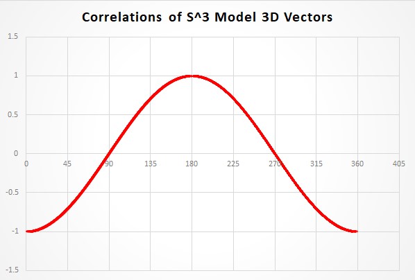
The plot of the data is very simple. The x axis is
Here is a link to the raw GAViewer data for 25K trials as a .csv file (about 500K file size). The first column is the angle and the second column is the correlation value at that angle.
EPRsims/newjoyGA3D25k2.csv
.
